Baker K.R. Optimization Modeling with Spreadsheets
Подождите немного. Документ загружается.

The critical sources correspond to binding supply constraints in the model. In the
solution, the Minnesota and Pittsburgh plants are at capacity, and Tucson capacity
is underutilized. The decision variables associated with Tucson as a source are not
determined by the capacity at Tucson; instead, they are determined by other constraints
in the model.
In summary, the structural scheme for the pattern is as follows.
†
Demands at all five warehouses are binding.
†
Capacities at Minnesota and Pittsburgh are binding.
†
The desired routes are MC, PA, PB, TA, TC, and TD.
As we shall see, this structural scheme specifies the optimal solution uniquely.
In the optimal schedule, some demands are met entirely from a unique source:
Demand at Boston is entirely met from Pittsburgh, and demand at Denver is entirely
met from Tucson. In a sense, these are high priority scheduling allocations, and we can
think of them as if they are made first. There is also a symmetric feature: Supply from
Minneapolis all goes to Chicago. Allocating capacity to a unique destination also
marks a high priority allocation.
It is tempting to look for a reason why these routes get high priority. At first
glance, we might be inclined to think that these are the cheapest routes. For example,
Boston’s cheapest inbound route is certainly the one from Pittsburgh. However, things
get a little more complicated after that. The TD route is not the cheapest inbound route
for Denver. Luckily, we don’t need to have a reason; our task here is merely to interpret
the result.
Once we assign the high priority shipments, we can effectively ignore the supply
at the Minneapolis plant and the demands at the Boston and Denver warehouses. We
then proceed to a second priority level, where we are left with a reduced problem con-
taining two sources and two destinations. Now, the list of best routes tells us that the
remaining supply at Pittsburgh must go to Atlanta; therefore, PA is a high priority allo-
cation in the reduced problem. Similarly, the remaining demand at Chicago is entirely
met from Tucson, so the TC route becomes a high priority allocation as well.
Having made the second-priority assignments, we can ignore the supply at
Pittsburgh and the demand at Chicago. We are left with a net demand at Atlanta
and unallocated supply at Tucson. Thus the last step, at the third priority level, is to
meet the remaining demand with a shipment along route TA.
In general, the solution of a transportation problem can be described with the
following generic computational scheme.
†
Identify a high priority demand—one that is met from a unique source—and
allocate its entire demand to this route. Then remove that destination from
consideration.
†
Identify a high priority source—one that supplies a single destination—and
allocate its remaining supply to this route. Then remove that source from
consideration.
146
Chapter 4 Sensitivity Analysis in Linear Programs

†
Repeat the previous two steps using remaining demands and remaining
supplies each time until all shipments are accounted for.
The specific steps in the computational scheme for our example are the following.
1. Ship as much as possible on routes PB, TD, and MC.
2. At the second priority level, ship as much as possible on routes PA and TC.
3. At the third priority level, ship as much as possible on route TA.
At each allocation, “as much as possible” is dictated by the minimum of capacity
and demand. The following list summarizes computational scheme in priority order.
Route Priority Shipment
PB 1 10,000
TD 1 9000
MC 1 10,000
PA 2 5000
TC 2 2000
TA 3 3000
This retrospective calculation of the solution has two important features: It is complete
(i.e., it specifies the entire shipment schedule) and it is unambiguous (i.e., the calcu-
lation leads to just one schedule). Anyone who constructs the solution using these
steps will reach the same result.
The structural scheme given earlier characterizes the optimal solution without
explicitly using a number. By describing the optimal solution without relying on
the specific parameters in the problem, it portrays a qualitative pattern in the solution.
Then, by converting that pattern to a computational scheme, we translate the pattern
into a list of economic priorities. This list enables us to establish the values of the
decision variables one at a time.
This pattern is important because it holds not just for the specific problem that we
solved, but also for other problems that are very similar but with some of the para-
meters slightly altered. For example, suppose that demand at Boston were raised to
10,500. We could verify that the same pattern applies. The revised details of imple-
menting the same pattern are shown in the following list.
Route Priority Shipment Change D Cost
PB 1 10,500 500 150
TD 1 9000 0 0
MC 1 10,000 0 0
PA 2 4500 –500 – 180
TC 2 2000 0 0
TA 3 3500 500 325
4.6. Patterns in Linear Programming Solutions
147

Summing the cost changes in the last column, we find that an increase of 500 in
demand at Boston leads to an increase in total cost of $295. In effect, we have derived
the shadow price because the per-unit change in total cost would be $295/500 ¼
$0.59. This value agrees with the shadow price for Boston demand given in the
Sensitivity Report (Figure 4.15).
In tracing the changes, we can also anticipate the range over which the shadow
price continues to hold. As we add units to the demand at Boston, the pattern
induces us to make the same incremental adjustments in shipment quantities we
traced in the table above. The pattern of shipments will be preserved, and the list
of best routes will remain unaltered, as long as we add no more than 1000 units
to the demand at Boston. At that level, the excess capacity in the system disappears,
and the pattern no longer holds. In the other direction, as demand at Boston drops,
the pattern indicates that we should reduce shipments on PB and TA, while increas-
ing PA. After we have reallocated 3000 units in that way, the allocation on route TA
disappears. At that point, we have to shift to a new pattern to accommodate a further
drop in Boston demand. The limits found here—an increase of 1000 and a decrease
of 3000—are precisely the limits on the Sensitivity Report for Boston demand.
Thus, using the optimal pattern, we are able to explain the shadow price and its
allowable range.
More generally, we can alter the original problem in several ways at once.
Suppose demands at Atlanta, Boston, and Chicago are each raised by 100 simul-
taneously. What will the optimal schedule look like? In qualitative terms, we already
know from the computational scheme. The qualitative pattern allows us to write down
the optimal solution to the revised problem without re-running Solver, but rather by
using the priority list and adjusting the shipment quantities for the altered demands.
The following table summarizes the calculations.
Route Priority Shipment Change D Cost
PB 1 10,100 100 30
TD 1 9000 0 0
MC 1 10,000 0 0
PA 2 4900 – 100 –36
TC 2 2100 100 55
TA 3 3200 200 130
Tracing the cost implications, we find that the 100-unit increases in the three
demands combine to increase the optimal total cost by $179. This figure can be
obtained by adding the three corresponding shadow prices (and multiplying by the
size of the 100-unit increase), but the pattern allows us to take one additional step.
We can also determine that the $179 figure holds for an increase (in the combined
demand levels) of 1000, which is the level at which the excess supply disappears,
or for a decrease of 1500, which is the level at which the shipment along TA runs
out. Thus, we can find the allowable range for a shadow price corresponding to sim-
ultaneous changes in several constraint constants.
148
Chapter 4 Sensitivity Analysis in Linear Programs
4.6.2. The Product Portfolio Model
The product portfolio problem asks which products a firm ought to be making. If con-
tractual constraints force the firm to enter certain markets, then the question is which
products to make in quantities beyond the required minimum. Consider Grocery
Distributors (GD), a company that distributes 15 different vegetables to grocery
stores. GD’s vegetables come in standard cardboard cartons that each take up 1.25
cubic feet in the warehouse. The company replenishes its supply of frozen foods at
the start of each week and rarely has any inventory remaining at the week’s end. An
entire week’s supply of frozen vegetables arrives each Monday morning at the ware-
house, which can hold up to 18,000 cubic feet of product. In addition, GD’s supplier
extends a line of credit amounting to $30,000. That is, GD is permitted to purchase up
to $30,000 worth of product each Monday.
GD can predict sales for each of its 15 products in the coming week. This forecast
is expressed in terms of a minimum and maximum anticipated sales quantity. The
minimum quantity is based on a contractual agreement that GD has made with a
small number of retail grocery chains; the maximum quantity represents an estimate
of the sales potential in the upcoming week. The cost and selling price per carton
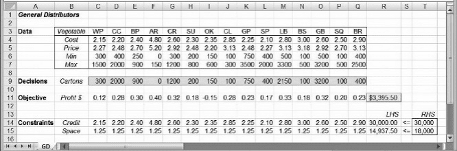
for each product are known. The given information is tabulated as part of Figure 4.19.
GD solves the linear programming model shown in Figure 4.19. The model’s
objective is maximizing profit for the coming week. Sales for each product are con-
strained by a minimum and maximum quantity. These are entered as lower and
upper bound constraints. In addition, aggregate constraints on purchase expenditures
and warehouse space make up the model. The model specification is as follows.
Objective: R11 (maximize)
Variables: C9:Q9
Constraints: R14:R15 T14:T15
Bounds: C9:Q9 C6:Q6 (lower bounds)
C9:Q9 C7:Q7 (upper bounds)
Figure 4.19 also displays the solution obtained by running Solver. When we look at the
constraints of the problem, we see that the credit limit is binding, but the space
Figure 4.19. Optimal solution for GD.
4.6. Patterns in Linear Programming Solutions 149
constraint is not. That means space consumption is dictated by other constraints in the
problem. When we look at demand constraints, we see that creamed corn, black-eyed
peas, carrots, and green beans are purchased at their maximum demands, whereas all
other products are purchased at their minimum, except for lima beans. This obser-
vation constitutes a first cut at the structural scheme in the optimal solution.
The pattern thus consists of a set of products produced at their minimum levels,
another set produced at their maximum levels, and the information that the credit limit
is binding. We can translate this pattern into a priority list by treating the products pro-
duced at their maximum levels as high priority products. The products produced
exactly at their minimum levels are the low priority products. Lima beans are in a
unique role. We can think of the solution as assigning the high priority products to
their maximum levels and the low priority products to their minimum levels. This
brings us to the only remaining positive variable—the lima beans. We assign their
quantity so that the credit limit becomes binding.
We can go one step further and recognize from the pattern that we are actually
solving a simpler problem than the original: Produce the highest possible value
from the 15 products under a tight credit limit. To solve this problem, we can use a
common-sense rule: Pursue the products in the order of highest value-to-cost ratio.
The only other consideration is satisfying the given minimum quantities. Therefore,
we can calculate the solution as follows.
1. Purchase enough of each product to satisfy its minimum quantity.
2. Rank the products from highest to lowest ratio of profit-to-cost.
3. For the highest-ranking product, raise the purchase quantity toward its maxi-
mum quantity. Two things can happen: Either we increase the purchase quan-
tity so that the maximum is reached (in which case we go to the next product),
or else we use up the credit limit (in which case we stop).
The ranking mechanism prioritizes the products and defines the computational
scheme for the pattern. Using these priorities, we essentially partition the set of pro-
ducts into three groups: a set of high priority products, produced at their maximum
levels; a set of low priority products, produced at their minimum levels; and a special
product, produced at a level between its minimum and its maximum. (The special pro-
duct is the one we are adding to the purchase plan in our computational scheme when
we hit the credit limit.) This procedure is complete and unambiguous, and it describes
the optimal solution without explicitly using a number. At first, the pattern was again
just a collection of positive decision variables and binding constraints. But we were
able to convert that pattern into a prioritized list of allocations—a computational
scheme—that established the values of the decision variables one at a time.
Table 4.2 summarizes the computational scheme. It ranks the products by profit-
to-cost ratio and indicates which products are purchased at either their maximum or
minimum quantity.
Actually, Solver’s solution merely distinguished the three priority classes; it did
not actually reveal the value-to-cost ratio rule explicitly. That insight could come from
150
Chapter 4 Sensitivity Analysis in Linear Programs

reviewing the make-up of the priority classes, or from some outside knowledge about
how single-constraint problems are optimized. But this brings up an important point.
Usually, Solver does not reveal the economic reason for why a variable is treated as
having high priority. In general, it is not always necessary (or even possible) to
know why an allocation receives high priority—it is important to know only that it
does.
As in the transportation example, we can alter the base-case model slightly and
follow the consequences for the optimal purchase plan. For example, if we raise the
credit limit, the only change at the margin will be the purchase of additional cartons
of the medium priority product. Thus, the marginal value of raising the credit limit
is equivalent to the incremental profit per dollar of purchase cost for the medium pri-
ority product, or (3.13 – 2.80)/2.80 ¼ 0.1179. Furthermore, we can easily compute
the range over which this shadow price continues to hold. At the margin, we are
adding to the 2150 cartons of lima beans, where each carton adds $0.1179 of profit
per dollar of cost. As we expand the credit limit, the optimal solution will call for
an increasing quantity of lima beans, until it reaches its maximum demand of 3300
cartons. Those extra (3300 – 2150) ¼ 1150 cartons consume an extra $2.80 each of
an expanded credit limit, thus reaching the maximum demand at an additional
2.80(1150) ¼ $3220 of expansion in the credit limit. This is exactly the allowable
increase for the credit limit constraint. For completeness, we should also check on
the other nonbinding constraint, because we ignored the space constraint in the pattern.
The extra 1150 cartons of lima beans consume additional space of (1.25)1150 ¼
1437.5 square feet of space. But this amount can be accommodated by the unused
Table 4.2. GD’s Products, Arranged by Priority
Product Priority Quantity Profit/cost
Creamed corn 1 2000 0.127 (max.)
Black-eyed peas 2 900 0.125 (max.)
Carrots 3 1200 0.123 (max.)
Green beans 3 3200 0.123 (max.)
Lima beans 4 2150 0.118 (spec.)
Green peas 5 750 0.102 (min.)
Cauliflower 6 100 0.098 (min.)
Spinach 7 400 0.081 (min.)
Squash 8 100 0.079 (min.)
Broccoli 9 400 0.079 (min.)
Succotash 10 200 0.078 (min.)
Brussel sprouts 11 100 0.060 (min.)
Whipped potatoes 12 300 0.056 (min.)
Okra 13 150 – 0.064 (min.)
4.6. Patterns in Linear Programming Solutions
151
space of 3063 square feet in the original optimal solution. This calculation confirms
that lima bean demand reaches its maximum level at the allowable increase of
$3220 in the credit limit.
Suppose we increase the amount of a low priority product in the purchase plan.
Then, following the optimal pattern (Steps 1–3 above), we would have to purchase
less of the medium priority product. Consider the purchase of more squash than the
100-carton minimum. Each additional carton costs $2.50, substituting for about
2.50/2.80 ¼ 0.893 cartons of lima beans in the credit limit constraint. The net
effect on profit is as follows.
†
Add a carton of squash (increase profit by $0.20).
†
Remove 0.893 cartons of lima beans (decrease profit by $0.2946).
†
Therefore, net cost ¼ $0.0946.
Thus, each carton of squash we force into the purchase plan (above the minimum of
100) will reduce profits by 9.46 cents, which corresponds to the reduced cost for
squash. Over what range will this figure hold? From the optimal pattern, we see that
we can continue to swap squash for lima beans only until the squash rises to its maxi-
mum demand of 500 cartons, or until lima beans drop to their minimum demand of
500 or until the excess space is consumed, whichever occurs first. The maximum
demand for squash is the tightest of these limits; thus, the reduced cost holds for
400 additional cartons of squash above its minimum demand, a figure that is not
directly accessible on the Sensitivity Report.
Comparing the analysis of GD’s problem with the transportation problem con-
sidered earlier, we see that the optimal pattern, when translated into a computational
scheme, is complete and unambiguous in both cases. We can also use the pattern to
determine shadow prices on binding constraints and the ranges over which these
values continue to hold; similarly, we can use the pattern to derive reduced costs
and their ranges as well. A specific feature of GD’s model is the focus on one particular
bottleneck constraint. This helps us understand the role of a binding constraint when
we interpret a pattern; however, many problems have more than one binding
constraint.
4.6.3. The Investment Model
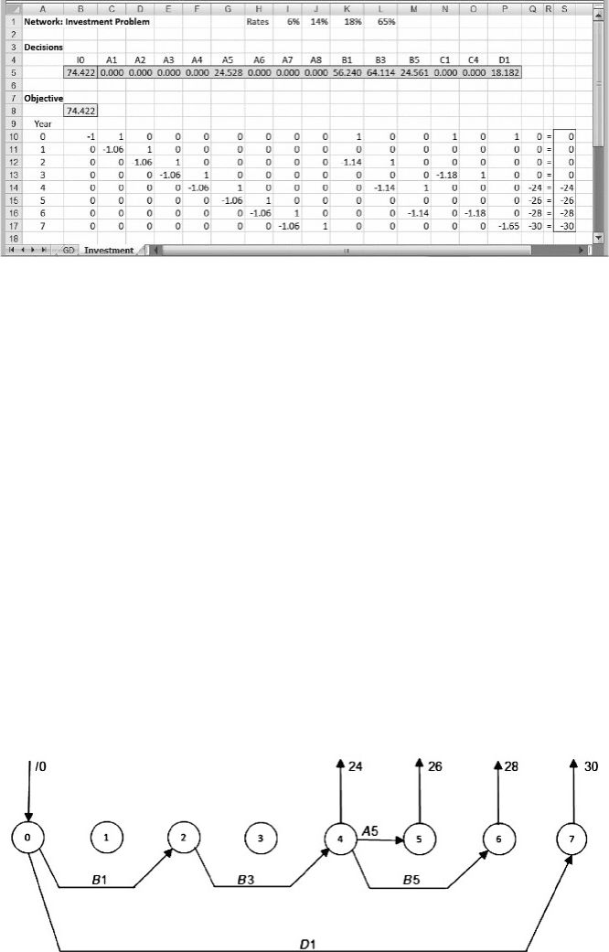
Next, let’s revisit Example 3.5, the network model for multiperiod investment. The
optimal solution is reproduced in Figure 4.20. Because it is a network, all the con-
straints are binding. Furthermore, six variables are positive in the optimal solution.
Therefore, the structural scheme for the pattern is to take every constraint as binding
and rely on the following list of variables: I0, A5, B1, B3, B5, and D1. The solution
tells us to ignore the other variables.
How can we use the constraints to dictate the values of the nonzero variables? One
helpful step is to recreate the network diagram, using just the variables known to be
part of the solution. Figure 4.21 shows this version of the network diagram.
152
Chapter 4 Sensitivity Analysis in Linear Programs
If we think of the cash outflows in the last four years of the model as being met by
particular investments, it follows that the last cash flow is met by either A7orD1.
These are the only investments that mature in year 7, but the structural scheme tells
us to ignore A7. From Figure 4.21, we can see that the size of D1 must exactly
cover the required outflow in year 7. Similarly, the candidates to cover the year 6
cash outflow are A6, B5, and C4. Of these, only B5 is nonzero, so B5 covers the
required outflow in year 6. The use of B5 also adds to the required outflow in year
4. For the required outflow in year 5, the only nonzero candidate is A 5, which also
adds to the required outflow in year 4. The combined year 4 outflows must be covered
by B3, which in turn imposes a required outflow in year 2, to be covered by B1.
Table 4.3 summarizes the calculations, working backward from year 7.
Working down this list, the investment in D1 is determined by the requirement in
year 7. The size of B5 is determined by the requirement in year 6, and similarly, the
size of A5 is determined by the requirement in year 5. These latter two investments
and the given outflow in year 4 together determine the investment in B3. (For that
reason, we need to know the size of B5 and A5 before we can calculate the size of
Figure 4.20. Optimal solution to Example 3.5.
Figure 4.21. Network model corresponding to Figure 4.21.
4.6. Patterns in Linear Programming Solutions 153

B3.) The size of B3, in turn, dictates the investment in B1. Finally, the sizes of B1 and
D1 determine how much money must be invested initially.
Once again, this description of the solution is complete (specifies the entire invest-
ment schedule) and unambiguous (leads to just one schedule). The binding constraints
and the positive decision variables, as displayed in Figure 4.21, describe a compu-
tational scheme for calculating the values of the decision variables one at a time, as
if following a priority list.
As in the other examples, we can obtain shadow prices by incrementing one of the
constraint constants and repeating the process. For example, if the last outflow changes
to $31,000 then, following the pattern, we know that the only change will be an
increase in D1, raising the initial investment. In particular, for an increased outflow
of $1000, D1 would have to be augmented by 1000/1.65 (because it returns 65 per-
cent) or $606.06. Thus, the shadow price on the last constraint is 0.606, as can be
verified by obtaining the Sensitivity Report for the base-case optimization run. To
determine the range over which this shadow price holds, we must calculate when
some nonbinding constraint becomes tight. For this purpose, the only nonbinding con-
straints we need to worry about are the nonnegativity constraints on the variables,
because each of the formal constraints in the model is an equality constraint already.
The shadow price on the last constraint therefore holds for any increase in the size of
the last outflow.
4.6.4. The Allocation Model
In the examples discussed thus far, the pattern led us to a way of determining the vari-
ables one at a time, in sequence. After one variable in this sequence was determined,
we had enough information to determine the next one, and we could continue until all
of the positive variables were determined. Not all solutions lead to this sequential list-
ing, however. As an example, let’s revisit the allocation model, shown in Figure 4.7.
When we ignore the zero-valued variables and the nonbinding constraints, we are
left with a structural scheme consisting of two binding constraints (for assembly and
machining capacity) and two positive variables (desks and tables). There is only one
way that a product mix of desks and tables can be chosen to precisely consume all
assembly and machining capacity. To find that mix, we must solve the following
Table 4.3. Computational Scheme for the Investment Model
Year Outflow Met by Rate Inflow at year
7 30,000 D1 65% 18,182 at 1
6 28,000 B5 14% 24,561 at 4
5 26,000 A5 6% 24,528 at 4
4 73,089 B3 14% 64,114 at 2
30
2 64,114 B1 14% 56,240 at 1
1 74,422 I0–
154 Chapter 4 Sensitivity Analysis in Linear Programs
two equations in two unknowns.
8D þ 6T ¼ 2000
6D þ 4T ¼ 1440
The unique solution to the two equations is D ¼ 160 and T ¼ 120, which is com-
plete and unambiguous for the model. Thus, in this example, we cannot create a pri-
ority list for calculating the variables one at a time. Instead, our computational scheme
amounts to the solution of a pair of equations, allowing us to compute the values of the
two positive variables simultaneously.
Because this is not a difficult system to solve for specific values of D and T, we can
also solve it parametrically. Let A and M denote the assembly and machining
capacities, respectively. Then the solution is
D ¼ (3M 2A)=2
T ¼ (3A 4M)=2
This form allows us to evaluate shadow prices easily. For example, if we increase M by
a unit amount, D increases by 1.5, T decreases by 2, and the objective function
increases by
DProfit ¼ 20D þ 14T ¼ 20(1:5) þ 14(2) ¼ 30 28 ¼ 2
We recognize the $2 shadow price from earlier analysis (Figure 4.16).
We can also use the parametric form to derive the allowable range. Again,
suppose we increase M. From the parametric solution, we see that D will increase,
but T will drop. The combination also increases the consumption of fabrication
hours and wood supply. The pattern will last until T drops to zero, fabrication becomes
binding or wood becomes binding, whichever occurs first. It turns out that the first
change in the pattern comes from wood. Recall that the wood constraint is
40D þ 25T 9600
Using the parametric solution in our pattern, this expression becomes
40(3M 2A)=2 þ 25(3A 4M)=2 ¼ 10M 2:5A 9600
or, with A ¼ 2000
10M 14,600
Therefore, the pattern holds until M ¼ 1460, which corresponds to an allowable
increase of 20.
4.6.5. The Refinery Model
To repeat the main idea: When we specify the structural scheme for a pattern in the
optimal solution, we focus on the decision variables that are positive and the con-
straints that are binding. In effect, we ignore zero-valued variables and nonbinding
constraints. As a final illustration, we revisit the refinery model of Example 3.6 for
4.6. Patterns in Linear Programming Solutions 155