Baker K.R. Optimization Modeling with Spreadsheets
Подождите немного. Документ загружается.

The table shows how Pittsburgh shipments and the optimal total cost change as
Pittsburgh’s capacity varies. The columns correspond to the same outputs that were
selected for the previous table, except that the parameter we’ve varied (Pittsburgh
capacity) appears in the first column. The rows correspond to the designated series
of input values for this parameter. (For Pittsburgh capacities below 14,000, the optim-
ization problem would be infeasible. At those levels, capacity in the system would be
insufficient to meet demand for 39,000 units.) In the table, the following changes
appear in the optimal schedule.
†
As Pittsburgh’s capacity increases above 14,000, total costs drop, and more
shipments occur on the PA route.
†
When Pittsburgh’s capacity reaches 18,000, shipments along PA level off at
8000. Beyond that capacity level, the solution uses the PC route.
†
The optimal total cost drops as Pittsburgh’s capacity increases to 20,000.
Beyond that level, the optimal schedule stabilizes, and total cost remains at
$12,420.
Thus, if we can find a way to increase the capacity at Pittsburgh, we should be inter-
ested in an increase up to a level of 20,000 from the base-case level of 15,000. By also
investigating the cost of increasing capacity, we can quantify the net benefits of expan-
sion. If there are incremental costs associated with expansion to capacities beyond
20,000, such costs are not worth incurring because there is no benefit (i.e., no
reduction in total cost) when capacity exceeds that level. With this kind of information,
we can determine whether a proposed initiative to expand capacity would make econ-
omic sense.
Suppose, for example, that the Pittsburgh warehouse contained some excess space
that we could begin to use for just the cost of utilities. Furthermore, suppose this space
corresponded to additional capacity of 3000 units and cost $800 to operate. Would it
be economically advantageous to use the space? From the Parameter Analysis Report
we learn that by adding 3000 units of capacity, and operating with a capacity of 18,000
at Pittsburgh, distribution costs would drop to $12,960, a saving of $870 from the base
case. This more than offsets the incremental cost of utilities, making the use of the
space economically attractive.
The marginal value of additional capacity is defined as the change in the objective
function due to a unit increase in the capacity available (in this instance, an increase
of one in the value of Pittsburgh’s capacity). Starting with the base case, we can cal-
culate this marginal value by changing the capacity from 15,000 to 15,001, re-solving
the problem and noting the change in the objective function: Total cost drops to
$13,829.71, a decrease of $0.29.
To pursue this last point, we examine the column labeled Change in Figure 4.6.
Entries in this column equal the marginal value of Pittsburgh’s capacity. For example,
the first entry, in cell C3, corresponds to the ratio of the cost change (14,120–13,830)
to the capacity change (15,000 –14,000), or –0.29. As the table shows, the marginal
value starts out at $0.29, drops to $0.27, and eventually levels off at zero. Because the
table is built with increments of 1000, we get at least a coarse picture of how the
126
Chapter 4 Sensitivity Analysis in Linear Programs
marginal value behaves. To refine this picture, we would have to create a Parameter
Analysis Report with increments smaller than 1000.
As Pittsburgh’s capacity increases, the marginal value stays level for a while, then
drops, stays level at the new value for a while, then drops again. This pattern is an
instance of the economic principle known as diminishing marginal returns: If some-
one were to offer us more and more of a scarce resource, its value would eventually
decline. In this case, the scarce resource (binding constraint) is Pittsburgh’s capacity.
Limited capacity at Pittsburgh prevents us from achieving an even lower total cost; that
is what makes Pittsburgh’s capacity economically scarce.
Starting from the base case—15,000 hours—we should be willing to pay up to
$0.29 for each additional unit of capacity at the Pittsburgh plant. This value is also
called the shadow price. In economic terms, the shadow price is the break-even
price at which it would be attractive to acquire more of a scarce resource. In other
words, imagine that someone were to offer us additional capacity at Pittsburgh
(e.g., if we could lease some automated equipment). We can improve total cost at
the margin by acquiring the additional capacity, as long as its price is less than
$0.29 per unit. In our example of opening up additional space in the warehouse, the
cost of the addition was only $800/3000 ¼ $0.26. This figure is less than the
shadow price, indicating that it would be economically attractive to use the space.
Figure 4.6 shows that the marginal value of a scarce resource remains constant in
some neighborhood around the base-case value. In this example, the $0.29 shadow
price holds for additional capacity up to 18,000 units; then it drops to $0.27.
Beyond a capacity of 20,000 units, the shadow price remains at zero. In effect,
additional capacity beyond 20,000 units has no incremental value.
A distinct pattern appears in sensitivity tables when we vary the amount of a
scarce capacity. The marginal value of capacity remains constant over some interval
of increase or decrease. Within this interval, some of the decision variables change lin-
early with the change in capacity, while other decision variables may stay the same.
There is no interval, however, in which all the decision variables remain the same,
as is the case when we vary an objective function coefficient. Thus, it is the shadow
price—not the set of decision variables—that is insensitive to changes in the
amount of a scarce capacity in some interval around the base case. Beyond that
range, the story is different. If someone were to continually give us more of a
scarce resource, its value would drop and eventually fall to zero. In the case of our
transportation example, we can see in Figure 4.6 that the value of additional capacity
at Pittsburgh drops to zero at a capacity level of about 21,000.
4.2. PARAMETER ANALYSIS IN THE ALLOCATION
EXAMPLE
As a further illustration of the Parameter Analysis Report, let’s revisit Example 2.1 of
Chapter 2 (Brown Furniture Company) and the model that finds the profit-maximizing
product mix among chairs, desks, and tables. We encountered the optimal solution in
Figure 2.6, which is reproduced in Figure 4.7. The optimal product mix is made up of
4.2. Parameter Analysis in the Allocation Example 127
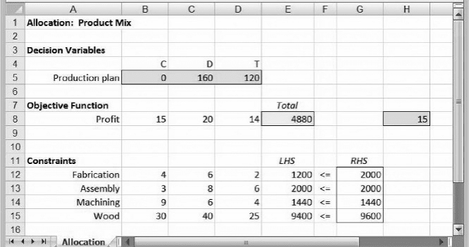
desks and tables, with no chairs; and the tight constraints are assembly and machining
hours. The optimal total profit contribution in the base case is $4880.
Suppose that we are using the allocation model as a planning tool and that we wish
to explore a change in the price of chairs. This price may still be subject to revision,
pending more information about the market, and we want to study the impact of a
price change, which translates into a change in the profit contribution of chairs. For
the time being, we’ll assume that if we vary the price, there will be no effect on the
demand potential for chairs. To explore the effect of a price change, we follow the
steps introduced in the previous section.
First, we designate a cell for the sensitivity information, in this case cell H8. We
enter the formula
=PsiOptParam(15,35), anticipating that we’ll want to investi-
gate the range of profit contributions from $15 to $35 per unit. We also enter a refer-
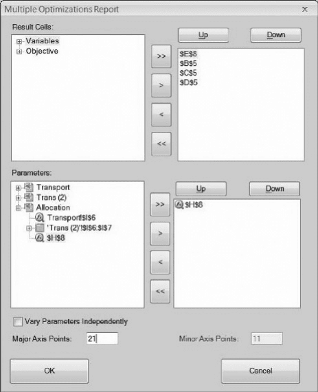
ence to H8 in cell B8. Next, we go to the drop-down menu for Reports on the RSP tab
and select Optimization
Q Parameter Analysis. In the top portion of the Multiple
Optimizations Report window, we select the objective function and variables in the
model, placing the objective function cell (E8) at the top of the list. Next, we select
H8 as the parameter cell, being careful to select it from the Allocation worksheet if
other worksheets appear on the list (because of the fact that they also contain the
PsiOptParam function). Then, by selecting 21 Major Axis Points, as shown in
Figure 4.8, we can examine the effects on a grid with $1 increments. The report,
with some reformatting, is tabulated in Figure 4.9.
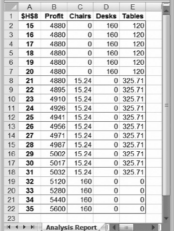
The first column of the table gives the values of the parameter (profit contribution
for chairs) that we varied. The second column lists the optimal value of the objective
function in each case and the third column calculates the rate of change in the objective
function per unit change in the parameter. These three columns are, again, the standard
part of the report. The last three columns in Figure 4.9 give the optimal values of the
three decision variables corresponding to each choice of the input parameter.
Figure 4.7. Optimal solution to Example 2.1.
128 Chapter 4 Sensitivity Analysis in Linear Programs
The Parameter Analysis Report shows how the optimal profit and the optimal pro-
duct mix both change as the profit contribution for chairs increases. For the selected
range of profit contributions ($15-$35), we see three distinct profiles. For values up
to $21, the base case solution prevails, but above $21, the optimal mix changes.
†
Chairs stay at zero until the unit profit on chairs rises to $21; then chairs enter
the optimal mix at a quantity of about 15.
†
When the unit profit reaches $32, the number of chairs in the optimal mix
increases to 160. At this stage, and beyond, the optimal product mix is made
up entirely of chairs.
†
Desks are not affected until the unit profit on chairs rises to $21; then the
optimal number of desks drops from 160 to 0.
†
Tables stay level at 120 until the unit profit on chairs rises to $21; then the opti-
mal number of tables increases to about 326. When the unit profit on chairs
rises to $32, the optimal number of tables drops to 0.
†
The optimal total profit remains unchanged until the unit profit on chairs rises
to $21; then it increases at a rate that reflects the number of chairs in the
product mix.
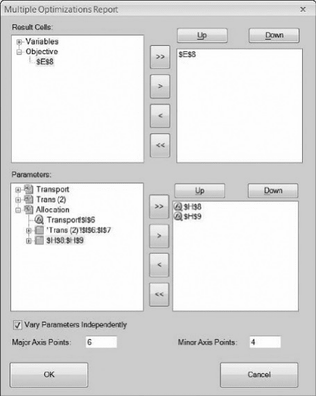
Figure 4.8. Selections in the Multiple Optimizations Report.
4.2. Parameter Analysis in the Allocation Example 129
From this information, we can conclude that the optimal solution is insensitive
to changes in the unit profit contribution of chairs, up to about $21. (Because we
are operating with a grid of $1, we do not have visibility into what might happen at
intermediate values.) Beyond that point, however, the profit on chairs would
become sufficiently attractive that we would want to include chairs in the mix. In
effect, chairs (and additional tables) substitute for desks when the profit contribution
of chairs reaches $21. Subsequently, when the profit contribution reaches $32,
additional chairs also substitute for tables. Thus, if we decide to alter the price for
chairs, we can anticipate the impact on the optimal product mix from the information
in the Parameter Analysis Report.
Again, the table illustrates some general qualitative patterns. First, when we
improve the objective function coefficient of one variable, the amount of that variable
in the optimal solution will either increase or stay the same; it cannot drop. (The effect
on other variables, however, may not follow an obvious direction: The optimal number
of tables first increases and then later decreases as the price of chairs rises.) Second, the
optimal value of the objective function either stays the same or improves.
Now let’s restore the model (by changing B8 back to 16) and consider one of
the RHS constants for sensitivity analysis instead of an objective function coefficient.
Starting from the base case, suppose we wish to vary the number of machining hours
available from 1200 to 2000 in steps of size 50, or equivalently 17 steps. We select
cell H9 for sensitivity parameters and enter
=PsiOptParam(1200,2000). Then
we reference H9 in cell G14, which holds the number of machining hours, and com-
plete the Multiple Optimizations Report, requesting 17 Major Axis Points.
Figure 4.9. Parameter Analysis Report for chair profit contribution.
130 Chapter 4 Sensitivity Analysis in Linear Programs
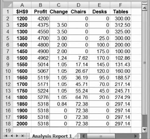
The Parameter Analysis Report (see Figure 4.10) shows how the optimal profit
and the optimal decisions both change as the number of machining hours increase.
The columns correspond to the same outputs as in the previous table, except for the
first column, where the rows correspond to the designated input values for machining
capacity. The table reveals the following changes in the optimal product mix.
†
Chairs remain out of the product mix until the number of machining hours rises
to about 1500. After that, chairs increase with the number of machining hours.
At around 1850 machining hours, the number of chairs levels off at about 72.4.
†
Desks increase as the number of machining hours rises to about 1450; then
desks decrease. At 1850 machining hours, desks drop out of the optimal mix.
†
Tables make up the entire product mix until the number of machining hours
rises to about 1350. Then the optimal number of tables first decreases, then
increases, and eventually levels off at about 297.
†
The optimal total profit grows as the number of machining hours rises, even-
tually leveling off at $5318.
Therefore, as we increase machining capacity above the base-case value of
1440, we have an incentive to alter the product mix. First, the product mix changes
by swapping desks for tables (but not necessarily at a ratio of 1: 1), then by swapping
chairs and tables for desks, until the entire product mix becomes devoted to chairs and
tables. The qualitative details of the product mix changes are not as important as the
fact that the optimal profit contribution increases with the number of machining hours,
until leveling off at a capacity of about 1850 hours.
Figure 4.10. Parameter Analysis Report for machining hours.
4.2. Parameter Analysis in the Allocation Example 131
We say “about” 1850 hours because we used a coarse grid in the table, and we
cannot observe precisely what machining capacity drives desks completely out of
the product mix. If we wanted a more precise value, we would repeat the analysis
using a step size less than 50.
The marginal value of additional machining hours is defined as the improvement
in the objective function from a unit increase in the number of hours available
(i.e., an increase of one in the right-hand side of the machining hours constraint).
Starting with the base case, we can calculate this marginal value, or shadow price,
by changing the number of machining hours to 1441, re-solving the problem, and
tracking the improvement in the objective function. (It grows to $4882, an improve-
ment of $2.)
In Figure 4.10, column C tracks the shadow price over a broader interval, based
again on a formula added manually to the table as it was originally generated. Entries
in this column represent the change in the optimal objective function value, from the
row above, divided by the change in the input parameter. This ratio describes the mar-
ginal value of machining hours. As the table shows, the marginal value starts out at
$3.50 for a capacity of 1250 machining hours, drops as the number of machining
hours increases, and eventually levels off at zero. Actually, the shadow price appears
to level off at $2.00 and at $1.05 before it eventually drops to zero. However, because
the table is built on increments of 50 hours, we can get only a coarse picture of how this
marginal value behaves.
To get a better picture of the marginal value, we can repeat the analysis, using a
step size of 25. The Parameter Analysis Report is shown in Figure 4.11. The marginal
values are still approximate; however, a clearer picture of the marginal value emerges.
As before, the marginal value lies at $3.50 at around 1200 hours; it falls to $2.00
around 1350 hours, to $1.05 around 1475 hours, and finally to zero around 1850
hours. An even smaller step size would be necessary to be more precise about the
levels at which the marginal value changes.
In linear programs, a distinct pattern in sensitivity analyses typically arises when
we vary the availability of a scarce resource. To repeat, the marginal value of the scarce
resource stays constant over some interval of increase or decrease. Within this interval,
some of the decision variables change linearly with the change in resource availability,
while other decision variables may stay the same. As we acquire more of a scarce
resource, its value eventually drops, exhibiting diminishing marginal returns and ulti-
mately falling to zero. In the case of our allocation problem, the value of additional
machining hours drops to zero at a capacity level around 1850.
For another perspective on this phenomenon, we can construct a graph of optimal
profit as a function of machining capacity. Figure 4.12 shows such a graph, with a dis-
tinctive piecewise linear shape. Machining capacity appears on the horizontal axis,
and optimal profit appears on the vertical axis. The slope of the line in this graph cor-
responds to the shadow price for machining capacity. As the graph indicates, the
shadow price drops in a piecewise fashion as the capacity increases, eventually stabi-
lizing at zero for capacity levels above 1850. As machining capacity increases beyond
this level, the optimal profit levels off at $5318, limited by other constraints in the
model.
132
Chapter 4 Sensitivity Analysis in Linear Programs
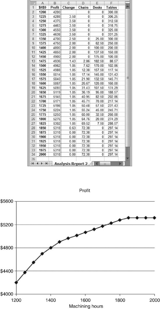
Figure 4.11. Parameter Analysis Report on a refined grid.
Figure 4.12. Optimal profit as a function of machining hours available.
4.2. Parameter Analysis in the Allocation Example 133
The Parameter Analysis Report has an option for generating two-way tables in
addition to the one-way tables we have examined thus far. For the two-way table,
we select two parameters and vary them from minimum to maximum, in a specified
step size. In other words, we enter the PsiOptParam function in two places and refer
to those functions in two cells of the model. (The ranges and step sizes need not be
identical.) The report generated by such a run displays only the values of the optimal
objective function.
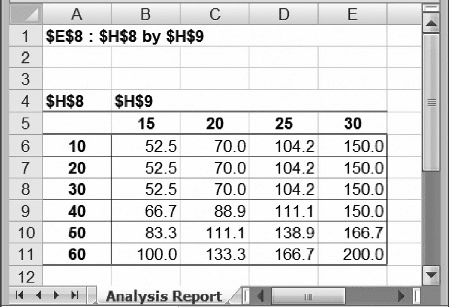
As an illustration, suppose we want to test the sensitivity of the optimal profit con-
tribution in the allocation example to changes in both the profit contribution of chairs
and the profit contribution of desks. Specifically, we vary the unit contribution of
chairs from 10 to 60 in steps of 10 and the unit contribution of desks from 15 to 30
in steps of 5. When we ask for a two-way table in the Multiple Optimizations
Report window, we check the box for Vary Parameters Independently and then
set the Major Axis Points to 6 and Minor Axis Points to 4 (for this illustration), as
shown in Figure 4.13. The Parameter Analysis Report is shown in Figure 4.14.
Although two-way tables are available, most sensitivity analyses are carried out
for one variable at a time. With a one-at-a-time approach, we can focus on the
Figure 4.13. Multiple Optimizations Report for a two-way analysis.
134 Chapter 4 Sensitivity Analysis in Linear Programs
implications of a change in a model parameter for the objective function, decision
variables, tightness of constraints, and marginal values. Much of the insight we
can gain from formal analysis derives from these kinds of investigations. The two-
at-a-time capability is computationally similar, but it does not usually provide as
much insight.
4.3. THE SENSITIVITY REPORT AND THE
TRANSPORTATION EXAMPLE
As we’ve seen, the Parameter Analysis Report duplicates for optimization models the
main functionality of the Data Table tool for basic spreadsheet models. The report is
constructed by repeating the optimization run with different parametric values in the
model each time. This transparent logic makes the Parameter Analysis Report a con-
venient and accessible choice for most of the sensitivity analyses we might want to
perform with optimization models. However, Solver provides us with an alternative
perspective.
The Sensitivity Report is available after an optimization run, once the optimal sol-
ution has been found. From the drop-down menu on the Reports icon in the RSP
ribbon, we select Optimization
Q Sensitivity. The Sensitivity Report then appears
on a new worksheet, immediately before the model worksheet. The Sensitivity
Report has three sections—one each for the objective function, decision variables,
and constraints. Figure 4.15 shows the Sensitivity Report for the transportation
model in Figure 4.1, after reformatting of some cells.
In the top section, the report records the optimal value of the objective function, as
it appears in cell C18. The report also guesses a suitable name for this quantity.
1
In the
Figure 4.14. Parametric Analysis Report for a two-way analysis.
1
By default, Solver constructs a name for each cell in this report by looking above it and to its left for text
entries in the original spreadsheet.
4.3. The Sensitivity Report and the Transportation Example 135