Baker K.R. Optimization Modeling with Spreadsheets

Подождите немного. Документ загружается.

second section, the report reproduces the values of the decision variables in the opti-

mal solution (under Final Value) and the values of the coefﬁcients in the objective

function (under Objective Coefﬁcient). The Allowable Increase and Allowable

Decrease columns show how much we could change any one of the objective function

coefﬁcients without altering the optimal decision variables. For example, the objective

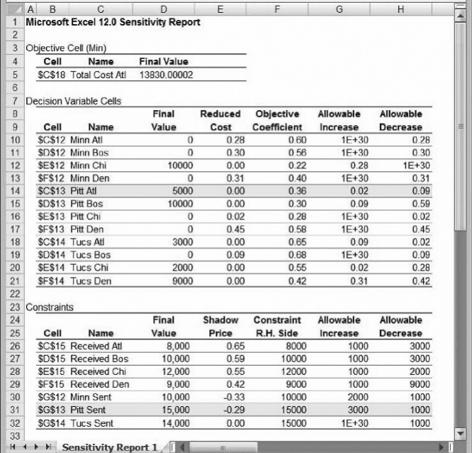
function coefﬁcient for the PA route is $0.36 in the base case, as shown in the ﬁrst

highlighted row of the Sensitivity Report in Figure 4.15. This unit cost could rise

to $0.38 without having an impact on the optimal shipping schedule. (This limit is

indicated by the allowable increase of 0.02.) In addition, the original value could

drop to $0.27 without having an impact on the optimal shipping schedule. (This

limit is indicated by the allowable decrease of 0.09.) These increases and decreases

from the base case are consistent with the parameter analysis shown in Figure 4.5.

It might be helpful to think about the Sensitivity Report as an “insensitivity

report,” because it mainly provides information about changes for which some

aspect of the base-case solution does not change. Here, for example, the base-case

Figure 4.15. Sensitivity Report for Example 3.1.

136 Chapter 4 Sensitivity Analysis in Linear Programs

decisions are insensitive to changes in the PA unit cost between $0.27 and $0.38. In

this interval, the base-case schedule remains optimal. Of course, the optimal total

cost will vary with the PA unit cost, because some 5000 units are shipped along the

PA route in the optimal schedule. For example, if the unit cost dropped by $0.04,

the optimal schedule would remain unchanged, but the optimal total cost would

drop by 5000($0.04) ¼ $200.

The Sensitivity Report is more precise but less ﬂexible than the Parameter

Analysis Report. For example, Figure 4.4 provides us with the allowable increase

and decrease, but to a precision of only 0.05. We need to search on a smaller grid,

as in Figure 4.5, to reﬁne our precision; but even in this more detailed report, we

can determine the allowable increase and decrease to a precision of only 0.01. By con-

trast, the Sensitivity Report provides the values exactly. On the other hand, the

Sensitivity Report tells us virtually nothing about what would happen if the PA unit

cost rose above $0.38, whereas the Parameter Analysis Report can provide a good

deal of information.

The entries in the Reduced Cost column of the Sensitivity Report may initially be

displayed as a set of zeros for all variables.

However, if we display the entries to two

decimal places, we see some nonzero values. For decision variables that are not at their

upper or lower bounds (and here, the only bound for a variable is zero), the reduced

cost is zero. So, for the variable PA, which is positive in the optimal shipping schedule,

the report shows a reduced cost of zero.

The reduced cost is nonzero if the corresponding decision variable lies at its

bound. In this example, that condition means that the route is not used in the optimal

schedule. For the MA route, the reduced cost is $0.28. The interpretation of this value

is as follows. Evidently, the unit cost of the MA route is unattractive at its base-case

value of $0.60, and we might wonder how much more attractive that unit cost

would have to become for the MA route to appear in the optimal solution. The

answer is given by the reduced cost: The unit cost would have to drop by more than

$0.28 before there would be an incentive to ship along the MA route. However, we

already knew that much, from the Allowable Decrease for the MA variable. As this

example shows, the Reduced Cost provides information that can be obtained else-

where, and we need not rely on it.

In the third section, the Sensitivity Report provides the values of the constraint

left-hand sides (under Final Value) and the right-hand-side constants (under

Constraint RH Side), along with the shadow price for each constraint. Here again, it

may be necessary to re-format the column of shadow prices. From the earlier sensi-

tivity analysis for this example, we expect to see a shadow price of $0.29 for

Pittsburgh capacity. The Sensitivity Report shows this value as a negative price

because it follows a convention of quoting the shadow price as the increase in the

objective function induced by a unit increase in the right-hand side constant. An

The format of these cells corresponds to the format of the corresponding decision cell in the original model.

Thus, depending on how the model was originally formatted, the ﬁgures in this report can be misleading,

especially when zeros appear.

4.3. The Sensitivity Report and the Transportation Example 137

increase in the Pittsburgh capacity would allow the optimal total cost to drop, so the

shadow price is negative.

The Allowable Increase and Allowable Decrease columns show how much we

could change any one of the constraint constants without altering the shadow price.

In the case of Pittsburgh capacity (15,000 in the base case), the information in the

highlighted row of the report’s bottom section indicates that the capacity could increase

by 3000 or decrease by 1000 (i.e., it could vary between 14,000 and 18,000) without

affecting the shadow price of $0.29. Again, this is an “insensitivity” result, and it is

consistent with the information in the Parameter Analysis Report of Figure 4.6.

Recall from our earlier discussions, however, that the optimal values of some decision

variables change with any increase or decrease in the Pittsburgh capacity.

The Sensitivity Report does not offer information about what occurs outside of

the allowable increase and allowable decrease. It is also completely based on one-

at-a-time analysis. That is, the presumption is that only one parameter at a time is

subject to change. No facility exists in the Sensitivity Report to explore the effects

of varying two parameters simultaneously, as in the case of the two-way parameter

analysis shown in Figure 4.14.

The sensitivity analysis for right-hand-side constants is omitted for constraints

that involve a simple lower or upper bound. That is, if the form of the constraint is

Variable  Ceiling or Variable  Floor, then the Sensitivity Report does not include

the constraint. On the other hand, if the same information is incorporated into the

model using the standard SUMPRODUCT constraint form (as in the case of the allo-

cation model) or using the SUM constraint form (as in the case of the transportation

model) then the Sensitivity Report treats the constraint in its usual fashion and pro-

vides ranging analysis.

4.4. THE SENSITIVITY REPORT AND THE

ALLOCATION EXAMPLE

As another illustration of the Sensitivity Report, suppose we ask for it after solving

Example 2.1, the allocation problem discussed earlier. (Refer to Figure 4.7, but

with the original proﬁt coefﬁcient of 16 restored to cell B8.) The Sensitivity Report

is shown in Figure 4.16. In the ﬁrst section, the report shows the optimal value of

the objective function (total proﬁt) of $4,880. In the second section, the Sensitivity

Report reproduces the optimal solution and tabulates the Allowable Increase and

Allowable Decrease for each objective function coefﬁcient. If we ask how much the

contribution of chairs ($16 in the base case) could vary without altering the optimal

product mix, we can tell from the ﬁrst Allowable Increase that the contribution

could rise by up to $5 or drop by any amount without altering the optimal mix.

Thus, a price increase of more than $5 would provide an inducement to include

chairs in the product mix. This conclusion could also be drawn from the parameter

analysis in Figure 4.7.

Suppose instead that we ask a similar question about desks: How much could the

proﬁt contribution for desks ($20 in the base case) change, without altering the

138

Chapter 4 Sensitivity Analysis in Linear Programs

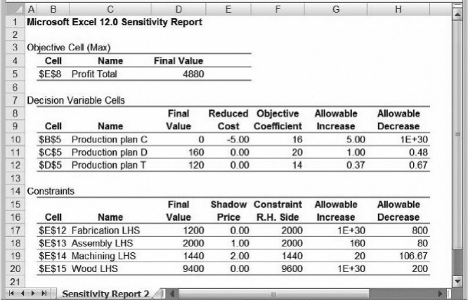
optimal solution? From the Sensitivity Report, in the row for desks, we see that the

allowable range is from $19.52 to $21.00 (from an Allowable Decrease of about

$0.48 to an Allowable Increase of $1.00). Within this interval, the unit proﬁt on

desks does not trigger a change in the optimal mix; the best mix remains 160 desks,

120 tables, and no chairs. However, any change outside this range should be examined

by re-running the model. Also, if the proﬁt on desks were to increase by $0.75, which

lies within the Allowable Increase, the optimal value of the objective function would

necessarily change because the 160 desks in the optimal mix would account for a proﬁt

increase of 160($0.75) ¼ $120.

The example involving the proﬁt on desks reinforces the point that the Sensitivity

Report cannot “see” beyond the Allowable Increase and Allowable Decrease. The

Sensitivity Report tells us nothing about what happens when the proﬁt contribution

for desks rises above $21, whereas that information would be available to us from

the Parameter Analysis Report, provided we specify a suitable range for the input

parameter. Nevertheless, the Sensitivity Report covers all of the decision variables

in one report. If we’re primarily interested in the allowable increases and decreases

around the base case—that is, if we’re looking for “insensitivity” information—

then the Sensitivity Report is the tool of choice. Had we used the Parameter

Analysis Report, we could not have produced information on all three coefﬁcients

simultaneously.

In the third section, the Sensitivity Report provides the shadow price for each con-

straint and the range over which it holds. The Allowable Increase and Allowable

Decrease columns show how much we could change any one of the constraint con-

stants without altering any of the shadow prices. For example, we should recognize

Figure 4.16. Sensitivity Report for Example 2.1.

4.4. The Sensitivity Report and the Allocation Example 139

the shadow price on Machining time of $2.00 (from Figure 4.11). However, from the

Sensitivity Report, we also know now that this $2.00 value holds up to a capacity

of 1460 hours (an allowable increase of 20). Beyond that, there would be a change

in the shadow price for machining hours. In fact, there would be a change in the

optimal product mix. Once again, we cannot anticipate from Sensitivity Report

exactly what that change might look like, whereas the Parameter Analysis Report

(Figure 4.11) shows that the expanded machining capacity will make it desirable to

add chairs to the product mix.

Thus, the Parameter Analysis Report and the Sensitivity Report provide different

capabilities. A comparison of the two approaches is summarized in Table 4.1.

Generally, the Parameter Analysis Report is more ﬂexible, whereas the Sensitivity

Report is more precise. Although each is suitable for answering particular questions

that arise in sensitivity analyses, it would be reasonable to draw on both capabilities

to build a comprehensive understanding of the model’s solution. One word of warning

must be added. The Sensitivity Report can sometimes be confusing if the model itself

does not follow a disciplined layout. As described in Chapter 2, we advocate a stan-

dardized approach to building linear programming models on spreadsheets. Solver

does permit more ﬂexibility in layout and calculation than our guidelines allow, but

some users ﬁnd the Sensitivity Report confusing when running nonstandard model

layouts. This problem is less likely to arise with the Parameter Analysis Report.

4.5. DEGENERACY AND ALTERNATIVE OPTIMA

Viewed from the perspective of the Sensitivity Report, each linear programming

solution carries with it an allowable range for the objective function coefﬁcients

Table 4.1. Comparison of the Parameter Analysis and Sensitivity Reports

Parameter Analysis Report Sensitivity Report

Differences

Describes user-determined region Describes “insensitivity” region

Can “see” beyond insensitivity region Limited to “insensitivity” region

Contains standard and tailored content Contains standard content

Table grid may need reﬁnements Allowable increase/decrease are precise

User may require several reports Information is provided simultaneously

Two-at-a-time analysis is available One-at-a-time analysis only

Any parameter on the worksheet Objective coefﬁcients and constraint constants

Similarities

Report is a new worksheet Report is a new worksheet

Column names may need revision Tabulated names may need revision

Entries in report table may need

reformatting

Entries in report table may need reformatting

140 Chapter 4 Sensitivity Analysis in Linear Programs

and RHS constants. Within this range, some aspect of the optimal solution remains

stable—decision variables in the case of varying objective function coefﬁcients and

shadow prices in the case of varying RHS constants. At the end of such a range,

the stability no longer persists, and some change sets in. In this section, we examine

the endpoints of these ranges as special cases.

First, let’s consider the allowable range for a constraint constant. For a particular

constraint, there is a corresponding range in which the shadow price holds. At the end

of that range, the shadow price is in transition, changing to a different value. At a point

of transition, a different shadow price holds in each direction. This condition is

referred to as a degenerate solution.

Consider our transportation example and its sensitivity report in Figure 4.15.

Suppose we are again interested in the analysis of Pittsburgh capacity, originally at

15,000. From the ranging analysis of Figure 4.15, we ﬁnd that the shadow price of

$0.29 holds for capacities of 14,000 to 18,000. At a capacity of 18,000, the shadow

price is in transition. We can see from Figure 4.6 that the shadow price is $0.29

below a capacity of 18,000 and $0.27 for capacities above it. Just at 18,000, it

would be correct to say that there are two shadow prices, provided that we also explain

that the 29-cent shadow price holds for capacity levels below 18,000, and a 27-cent

shadow price holds for capacity levels above 18,000. When we take capacity to be

exactly 18,000, however, Solver can display only one of these shadow prices. The

Sensitivity Report could show the shadow price either as $0.29 but with an allowable

increase of zero, or as $0.27 but with an allowable decrease of zero, depending on how

the model is expressed on the worksheet.

To recognize a degenerate solution, we look for an entry of zero among the allow-

able increases and decreases reported in the Constraints section of the Sensitivity

Report. This value indicates that a shadow price is at a point of transition. If none

of these entries is zero, then the solution is said to be a nondegenerate solution,

which means that no shadow price lies at a point of transition in the optimal solution.

The signiﬁcance of degeneracy is a warning: It alerts us to be cautious when using

shadow prices to help evaluate the economic consequences of altering a constraint

constant. We must be mindful that, in a degenerate solution, the shadow price holds

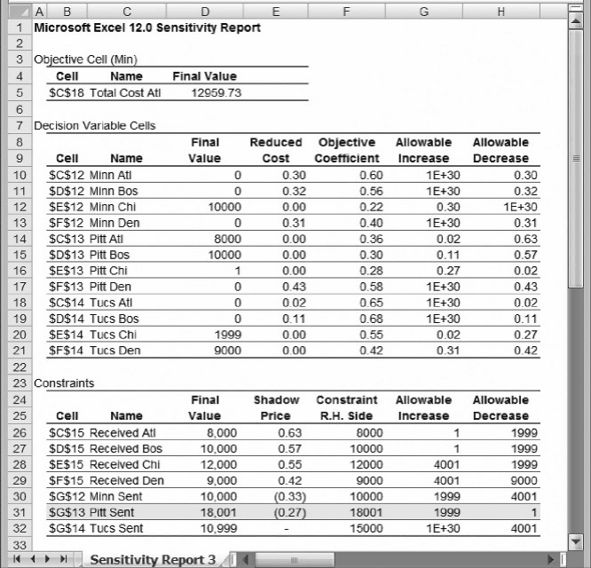
in only one direction. If we want to know the value of the shadow price just beyond

the point of transition, we can change the corresponding right-hand side by a small

amount and then re-run Solver. In our example, we could set Pittsburgh capacity

equal to 18,001 and re-optimize. The resulting Sensitivity Report reveals a 27-cent

shadow price for the Pittsburgh capacity constraint, along with an Allowable

Decrease of one, as shown in the highlighted row of Figure 4.17.

For a complementary result, suppose we have a problem that leads to a nonde-

generate solution, and we consider ranging analysis for objective function coefﬁcients.

For any particular coefﬁcient, there is a corresponding range in which the optimal

values of the decision variables remain unchanged. At the end of that range, more

than one optimal solution exists. This condition is referred to as alternative optima,

or sometimes multiple optima.

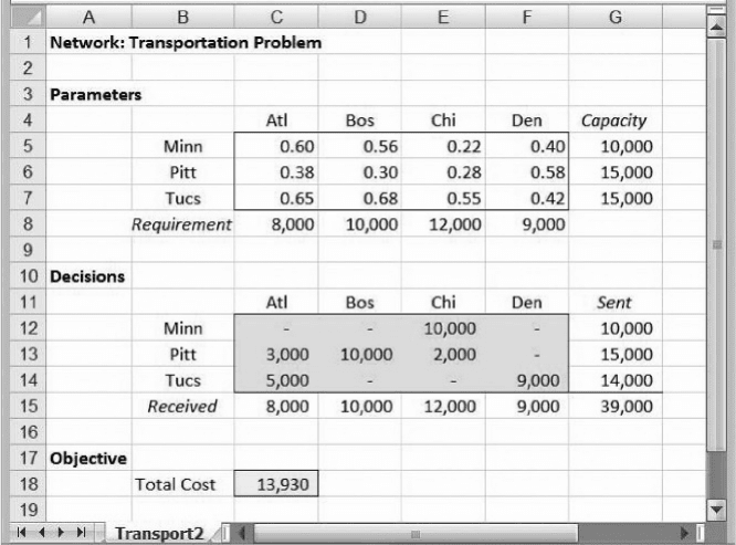
As an example, consider our original transportation model, as displayed in

Figure 4.1. From the ranging analysis of Figure 4.15, we see that the unit cost of the

4.5. Degeneracy and Alternative Optima 141

PA route can vary from $0.27 to $0.38 without a change in the optimal schedule. At the

38-cent limit of this range, more than one optimal solution exists. To ﬁnd this solution,

we change the unit cost on the PA route to 0.38 and re-run Solver. We ﬁnd that the

optimal total cost is $13,930, as shown in Figure 4.18. In this solution, the shipments

from Pittsburgh are 3000 to Atlanta, 10,000 to Boston and 2000 to Chicago, with cor-

responding adjustments to the Tucson shipments. However, we can verify that the

original optimal schedule generates this same total cost. In other words, we have

found two different schedules that achieve optimal costs. (In fact, it is possible to show

that any weighted average of the two schedules is also optimal; thus, the number of

distinct optimal schedules is actually inﬁnite.) Solver is able to display only one of

these solutions, depending on how the model is constructed on the spreadsheet.

To recognize the existence of multiple optima, we look for an entry of zero

among the allowable increases and decreases reported in the Decision Variable

Cells section of the Sensitivity Report. If there are no zeros, then the optimal solution

is a unique optimum, and no alternative optima exist. (Strictly speaking, this is true

Figure 4.17. Sensitivity Report for the near-degenerate case.

142 Chapter 4 Sensitivity Analysis in Linear Programs

only for nondegenerate solutions; when the solution is degenerate, these zeros are

not necessarily indicators of multiple optima.) Otherwise, the optimal solution

displayed on the spreadsheet is one of many alternatives that all achieve the same

objective function value. The signiﬁcance of multiple optima is an opportunity:

Knowing that there are alternative ways of reaching the optimal value of the objective

function, we might have secondary preferences that we could use as “tiebreakers” in

this situation. However, Solver does not have the capability of displaying multiple

optima, and it is not always obvious how to generate them on the spreadsheet. In

our example, we can at least “trick” Solver into displaying the original optimal

schedule for the case of a 38-cent unit cost on the PA route. If we change the unit

cost on the PA route to 0.37999 and re-run Solver, we obtain the output we desire.

Here, we exploit the fact that this made-up value remains inside the limits of the orig-

inal ranging analysis (as given in Figure 4.15), but it effectively behaves like the

desired parameter of 0.38.

In summary, the Sensitivity Report examines the objective function coefﬁcients

and the RHS constants separately in two tables. Taking each parameter independently,

and permitting it to vary, the report provides information on its allowable range—the

range of values for which the solution remains stable in some way. At the end of these

ranges, indicated by the values of the Allowable Increase and Allowable Decrease,

special circumstances apply. Box 4.1 summarizes the various conditions that can

occur when we start with an optimal solution that is unique and nondegenerate.

Figure 4.18. Solution with multiple optima.

4.5. Degeneracy and Alternative Optima 143

4.6. PATTERNS IN LINEAR PROGRAMMING

SOLUTIONS

We often hear that the real take-away from a linear programming model is insight,

rather than the actual numbers in the answer, but where exactly do we ﬁnd that insight?

This section describes one form of insight, which comes from interpreting the quali-

tative pattern in the solution. Stated another way, the optimal solution tells a “story”

about a pattern of economic priorities, and it’s the recognition of those priorities

that provides useful insight. When we know the pattern, we can explain the solution

more convincingly than when we simply transcribe Solver’s output. When we

know the pattern, we can also anticipate answers to some what-if questions without

having to modify the spreadsheet and re-run Solver. In short, the pattern provides a

level of understanding that enhances decision making. Therefore, after we optimize

a linear programming model, we should always try to describe the qualitative pattern

in the optimal solution.

BOX 4.1

Summary of Ranging in Sensitivity Analysis

Allowable ranges for objective function coefﬁcients

In the range from Allowable Increase to Allowable Decrease

†

the values of the decision variables remain the same

†

the binding constraints remain binding.

At the boundary of the range

†

multiple optima occur

†

the decision variables are in transition.

Inside the range (but not on its boundary)

†

the optimal set of decision variables is unique.

Allowable ranges for right-hand-side constants

In the range from Allowable Increase to Allowable Decrease

†

the shadow prices remain the same

†

the zero-valued decision variables remain zero.

At the boundary of the range

†

degeneracy occurs

†

the shadow price is in transition.

Inside the range (but not on its boundary)

†

the shadow prices are unique.

144 Chapter 4 Sensitivity Analysis in Linear Programs

Spotting a pattern involves making observations about both variables and con-

straints. In the optimal solution, we should ask ourselves, which constraints are bind-

ing and which are not? Which variables are positive and which are zero? A structural

scheme describing the pattern is simply a qualitative statement about binding con-

straints and positive variables. However, to make that scheme useful, we translate it

into a computational scheme for the pattern, which ultimately allows us to calculate

the precise values of the decision variables in terms of the model’s parameters. This

computational scheme often allows us to reconstruct the solution in a sequential,

step-by-step fashion. To the untrained observer, the computational scheme seems to

calculate the quantitative solution directly, without Solver’s help. In fact, we are pro-

viding only a retrospective interpretation of the solution, and we need to know that sol-

ution before we can construct the interpretation. Nevertheless, we are not merely

reﬂecting information in Solver’s output; we are looking for an economic imperative

at the heart of the situation depicted in the model. When we can ﬁnd that pattern and

communicate it, then we have gained some insight.

The examples in each of the subsections illustrate how to describe a pattern with-

out using numbers. The discussion also introduces two tests that determine whether

the pattern has been identiﬁed. We’ll see how knowledge of the pattern enables us

to anticipate the ranges over which shadow prices hold. We’ll also see how to antici-

pate the ranges over which reduced costs hold. In effect, this material amounts to an

explanation of information in the Sensitivity Report, although we can go beyond

the report. Ultimately, the ability to recognize patterns allows us to appreciate and

interpret solutions to linear programs in a comprehensive fashion, but it is a rather

different skill than using the Sensitivity Report. The identiﬁcation of patterns

allows us to look beyond the speciﬁc quantitative data of a problem and ﬁnd a general

way of thinking about the solution. Unfortunately, there is no recipe for ﬁnding

patterns—just some guidelines. The lack of a recipe can make the process challenging,

even for people who can build linear programming models quite easily. Therefore, our

discussion proceeds with a set of examples, each of which illustrates different aspects

of working with patterns.

4.6.1. The Transportation Model

Let’s return to the transportation example of Figure 4.1. The ﬁrst thing to notice is that

we need to use only six of the available routes in order to optimize costs. As Solver’s

solution reveals, the best routes to use are MC, PA, PB, TA, TC, and TD. Stated another

way, the solution tells us that we can ignore the other decision variables.

The solution also tells us that all the demand constraints are binding. This

makes intuitive sense because unit costs are positive on all routes, and so there is

no incentive to ship more than demand to any destination. A consequence of meeting

all demands exactly is that at least one of the supply capacities must be underutilized

in the optimal solution because there is a total demand of 39,000 units compared to a

total capacity of 40,000. In general, there is no way to anticipate how many sources

will be fully utilized and how many will be underutilized, so one useful part of

the optimal pattern is the identiﬁcation of critical sources—those that are fully utilized.

4.6. Patterns in Linear Programming Solutions 145