Baker K.R. Optimization Modeling with Spreadsheets
Подождите немного. Документ загружается.

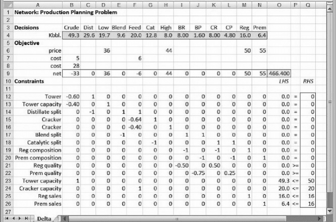
Delta Oil. The optimal solution is reproduced in Figure 4.22. Recall that the dimen-
sions for the variables in this model are thousands of barrels per day.
In the solution, all of the decision variables are positive, so the computational
scheme must determine each decision variable. When we look for binding constraints,
we find the balance equations, which define relationships among the decision vari-
ables, along with four others
†
Cracker capacity (at 20,000)
†
Reg sales (at 16,000)
†
Reg blend quality (at its floor of 50 percent Cat)
†
Prem blend quality (at its floor of 75 percent Cat).
In the computational scheme, these four binding constraints, together with the
definitional relationships in the balance equations, dictate the entire optimal solution.
We start with the cracker. Because the cracker is at its capacity limit, this means
Feed ¼ 20,000. Furthermore, the output of the cracker occurs in fixed proportions,
so it follows that Cat ¼ 12,800 and High ¼ 8000.
Next, we can use the fact that regular gasoline sells at its market limit, together
with the fact that it is blended at the minimum concentration of catalytic, to deduce that
BR ¼ 50% of 16,000 ¼ 8000
CR ¼ BR ¼ 8000
Figure 4.22. Spreadsheet model for Example 3.6.
156 Chapter 4 Sensitivity Analysis in Linear Programs

Now that we know Cat and CR, it follows from material balance considerations that
CP ¼ 4800.
Next, we use the fact that premium gasoline is blended at the minimum concen-
tration of catalytic, to deduce that
Prem ¼ 4800=(0:75) ¼ 6400
From material balance considerations, we have
BP ¼ Prem CP ¼ 6400 4800 ¼ 1600
We now know the allocation of the distillate blend, so
Blend ¼ BR þ BP ¼ 8000 þ 1600 ¼ 9600
Dist ¼ Blend þ Feed ¼ 9600 þ 20,000 ¼ 29,600
This calculation brings us back to the output of the tower, which we know is
60 percent distillate and 40 percent low-end by-products, yielding one last set of cal-
culations
Crude ¼ Dist=0:6 ¼ 29,600=0:6 ¼ 49,333
Low ¼ 0:4(Crude) ¼ 19,733
Thus, the optimal pattern calls for production that fully utilizes cracker capacity and
fully exploits sales potential for regular gasoline, while meeting minimum quality
levels in the blending of regular and premium gasolines. These qualitative constraints
represent the economic drivers that dictate the entire optimal solution.
Table 4.4. Computational Scheme for the Delta Oil Model
Base New
Variable case case Change
Feed 20,000 20,000
Cat 12,800 13,800 1000
High 8000 8000
BR 8000 8000
CR 8000 8000
CP 4800 5800 1000
Prem 6400 7733 1333
BP 1600 1933 333
Blend 9600 9933 333
Dist 29,600 29,933 333
Crude 49,333 49,889 556
Low 19,733 19,956 222
4.6. Patterns in Linear Programming Solutions
157
As we pointed out in Chapter 3, catalytic is a scarce resource at Delta Oil. If
more catalytic could be produced, Delta would be able to increase its profits. To
consider a specific scenario, suppose that a technological alteration of the cracker
could produce 1000 more barrels of catalytic without affecting the output of high-
end by-products. (In effect, this alteration modifies the original ratio of catalytic
output to feedstock input.) The following lists show the implications for the vari-
ables in the model. The base-case values come from the calculations illustrated
above; the new-case values in Table 4.4 are derived in a similar sequence, starting
with the fact that cracker capacity is fully utilized at 20,000 barrels and regular sales
are at the 16,000-barrel limit.
The economic implications follow from the objective function. Taking the vari-
ables that have nonzero coefficients in the objective function and evaluating the
impact of their changed values, we obtain
Profit ¼ 55(Prem) þ 36(Low) 33(Crude )
or
Profit ¼ 55(1333) þ 36(222) 33(556) ¼ 63,000
Thus, the alteration in cracker output could produce additional profits of $63,000 if
the production plan were adjusted optimally. On a per-unit basis, each barrel of
catalytic generated this way would produce $63 of additional profit. This figure
provides us with a tangible economic value for catalytic, which is an intermediate
product and which presumably has no market. However, if there were a market for
catalytic, we know that Delta would want to buy more catalytic at any price below
$63 per barrel.
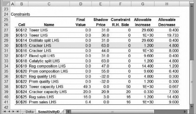
These calculations explain the shadow price on the first cracker constraint, which
defines catalytic in the linear programming model. An increase of one on the right-
hand side would be equivalent to setting Cat equal to one more than 40 percent of
the output from the tower. We can interpret this situation as equivalent to obtaining
one additional unit of Cat from an external source, as if it were freely available outside
of our technology. The shadow price tells us how much the objective function would
increase, per unit increase in the right-hand-side constant; and in the Constraints
section of the Sensitivity Report, we can verify that this value is 63, as shown in
Figure 4.23. Thus, our calculation exercise has essentially derived the shadow price.
More importantly, we can see how to use the optimal pattern to trace the economic
consequences of a technological change in the model.
One additional point is instructive. The $63 shadow price on catalytic has an
allowable increase of 1.2. Given the scaling convention in the model, this means
that the shadow price holds for an increase of only 1200 barrels of catalytic. To see
where this figure comes from, create a third column of figures in Table 4.4, starting
with a change in catalytic of 1200. The calculations lead to a Crude value of
50,000, meaning that the tower becomes fully utilized. Beyond that level, a new pat-
tern applies.
158
Chapter 4 Sensitivity Analysis in Linear Programs
SUMMARY
The primary role of Solver is to find solutions to optimization models. However, some of the
most useful information in the model comes from performing sensitivity analysis after the sol-
ution has been found. The information available through sensitivity analyses of linear programs
is elegant and comprehensive compared to what we find in other optimization techniques. In that
sense, the coverage in this chapter represents a kind of benchmark for the information we would
like to acquire in conjunction with an optimization analysis.
This chapter covered three approaches to sensitivity analysis: the Parameter Analysis
Report, the Sensitivity Report, and the interpretation of optimal patterns. The Sensitivity
Report is the most canned approach. It is a well defined report that complements the use of
Solver. Most importantly, it automatically reveals shadow prices and allowable ranges.
The Parameter Analysis Report allows the user quite a lot of flexibility, and it provides for
linear programs the same kind of capability that Excel’s Data Table tool provides for basic
spreadsheet models. The effects of modifying a parameter in the model can be traced well
beyond the range in the Sensitivity Report, and shadow prices can be computed in Excel when-
ever we vary a right-hand-side parameter.
The recognition of patterns in linear programming solutions is a way of looking beyond the
specific numbers in the result and toward a broader economic imperative. By focusing on posi-
tive variables and binding constraints, this interpretation emphasizes the key factors in the model
that drive the form of the solution. The ability to detect these factors sharpens our intuition and
enhances our ability to implement effective decisions based on the model.
The examples in Section 4.6 illustrate the process of extracting insight from the pattern in a
linear programming solution. The first step is to describe a structural scheme for the pattern by
examining the optimal decision variables and binding constraints. The more challenging step is
to convert this qualitative description into a computational scheme that allows us to “construct”
the optimal solution from the given parameters. Ideally, the computational scheme determines
Figure 4.23. Sensitivity Report (Constraints section) for Example 3.6.
4.6. Patterns in Linear Programming Solutions 159
the variables one at a time. This scheme can often be interpreted as a list of priorities, and those
priorities reveal the economic forces at work.
The pattern that emerges from the economic priorities is essentially a qualitative one, in
that we can describe it without using specific numbers. However, once we supply the parameters
of the constraints, the pattern leads us to the optimal quantitative solution. In a sense, it is almost
as if Solver first spots the optimal pattern and then says, “Give me the numerical information in
your problem.” For any specification of the numbers (within certain limits), Solver could then
compute the optimal solution by simply following the sequential steps in the pattern’s compu-
tational scheme. In reality, of course, Solver cannot know the pattern until the solution is deter-
mined, because the solution is a critical ingredient in the pattern.
Two diagnostic questions help determine whether we have been successful at extracting a
pattern: Is the pattern complete? Is it unambiguous? That is, the pattern must lead us to a full
solution of the problem, not just to a partial solution, and it must lead to a unique determination
of the variables. As a check on our specification of the pattern, we can derive shadow prices. In
each case, the shadow price comes from altering one constraint constant in the original problem.
We should be able to trace the incremental changes in the variables, through the various steps in
the pattern’s computational scheme, and ultimately derive the shadow price for the correspond-
ing constraint. We can also determine marginal values for changing several parameters at a time
in much the same way, and we can compute the allowable range over which these marginal
values continue to hold.
Unfortunately, it is not always the case that the pattern can be reduced to a list of assign-
ments in priority order. Occasionally, after we identify the positive variables and the binding
constraints in the optimal solution, we might be able to say no more than that the pattern
comes from solving a system of simultaneous equations determined by those constraints and
those variables. Nevertheless, in most cases, as the examples demonstrate, focusing on the pat-
tern can provide added insight beyond the numbers.
Patterns have certain limits, as suggested above. If we think of testing our specification of a
pattern by deriving shadow prices, we have to recognize that a shadow price has a limited range
over which it holds, as indicated by its allowable increase and allowable decrease. Beyond this
range, a different pattern prevails. As we change a constraint constant, the shadow price will
eventually change. The same is true of the pattern: Beyond the range in which the shadow
price holds, the pattern may change. In the product portfolio example, however, we were able
to specify the computational scheme in a general way, so that it holds even when the shadow
price changes. In that example, we were able to articulate the pattern at a high enough level
of generality that the qualitative “story” continues to hold even for substantial changes in the
given data.
EXERCISES
4.1. Transportation Patterns Revisited Revisit the transportation model of this chapter
and the pattern in its optimal solution.
(a) Suppose that Atlanta demand is increased by 100 units. Use the pattern to determine
the impact of this increase on the optimal total cost. What is the cost increase per unit
increase in demand at Atlanta? For how much of an increase in Atlanta demand will
this marginal cost continue to hold? Use the information in the Sensitivity Report to
confirm your results.
160 Chapter 4 Sensitivity Analysis in Linear Programs

(b) Repeat part (a) for a decrease of 100 units in Chicago demand.
(c) Repeat part (a) for an increase of 100 units in Minnesota capacity.
4.2. Product Portfolio Revisited Revisit the product portfolio model of this chapter and the
pattern in its optimal solution.
(a) Suppose that the credit limit of $30,000 is tightened. For each thousand-dollar
reduction, what is the impact on profit? Use the information in the Sensitivity
Report to confirm your results.
(b) Suppose that the minimum requirement for whipped potatoes is raised (above 300
cartons). Using the pattern, determine the impact of this demand increase on the
optimal profit. For how much of an increase in demand does this value hold?
Where does this information appear on the Sensitivity Report?
4.3. Distributing a Product The Lincoln Lock Company manufactures a commercial
security lock at plants in Atlanta, Louisville, Detroit, and Phoenix. The unit cost of pro-
duction at each plant is $35.50, $37.50, $37.25, and $36.25, and the annual capacities are
18,000, 15,000, 25,000, and 20,000, respectively. The locks are sold through wholesale
distributors in seven locations around the country. The unit shipping cost for each plant –
distributor combination is shown in the following table, along with the forecasted demand
from each distributor for the coming year.
Tacoma San Diego Dallas Denver St Louis Tampa Baltimore
Atlanta 2.50 2.75 1.75 2.00 2.10 1.80 1.65
Louisville 1.85 1.90 1.50 1.60 1.00 1.90 1.85
Detroit 2.30 2.25 1.85 1.25 1.50 2.25 2.00
Phoenix 1.90 0.90 1.60 1.75 2.00 2.50 2.65
Demand 5500 11,500 10,500 9600 15,400 12,500 6600
(a) Determine the least costly way of shipping locks from plants to distributors.
(b) List the shadow prices corresponding to each plant’s capacity. Which capacity has the
largest shadow price? For how large an increase does this value hold?
(c) Describe the qualitative pattern in the solution of part (a).
(d) Use the pattern in (c) to trace the effects of increasing the demands at Tacoma, San
Diego and Dallas by 100 simultaneously. How will the shipping schedule change?
What will be the change in the optimal total cost?
(e) For how much of a change in demand in part (d) will the pattern persist?
4.4. Make or Buy A sudden increase in the demand for smoke detectors has left Acme
Alarms with insufficient capacity to meet demand. The company has seen monthly
demand from its retailers for its electronic and battery-operated detectors rise to 20,000
and 10,000, respectively, and Acme wishes to continue meeting demand. Acme’s
production process involves three departments: Fabrication, Assembly and Shipping.
The relevant quantitative data on production and prices are summarized below.
Exercises
161

Monthly hours Hours/unit Hours/unit
Department available (electronic) (battery)
Fabrication 2000 0.15 0.10
Assembly 4200 0.20 0.20
Shipping 2500 0.10 0.15
Variable cost/unit $18.80 $16.00
Retail price $29.50 $28.00
The company also has the option of obtaining additional units from a subcontractor,
who has offered to supply up to 20,000 units per month in any combination of electronic
and battery operated models, at a charge of $21.50 per unit. For this price, the subcontrac-
tor will test and ship its models directly to the retailers without using Acme’s production
process.
(a) Determine how the manufacturer should allocate its in-house capacity and how it
should utilize the subcontractor. What are the maximum profit and the corresponding
make/buy levels? (This is a planning model; fractional decisions are acceptable.)
(b) Investigate the solution for Shipping capacities between 1200 and 2400 hours. Draw
a graph showing how the optimal quantities change over this range.
(c) Describe the qualitative pattern in the solution of part (a).
(d) Use the pattern in (c) to trace the effects of increasing the Fabrication capacity by
10%. How will the optimal make/buy mix change? How will the optimal profit
change?
(e) For how much of a change in Fabrication capacity will the pattern in (c) persist?
4.5. Selecting an Investment Portfolio An investment manager wants to determine an opti-
mal portfolio for a wealthy client. The fund has $2.5 million to invest, and its objective is
to maximize total dollar return from both growth and dividends over the course of the
coming year. The client has researched eight high-tech companies and wants the portfolio
to consist of shares in these firms only. Three of the firms (S1–S3) are primarily software
companies, three (H1 –H3) are primarily hardware companies, and two (C1 –C2) are
internet consulting companies. The client has stipulated that no more than 40 percent
of the investment be allocated to any one of these three sectors. To assure diversification,
at least $100,000 must be invested in each of the eight stocks.
The table below gives estimates from the investment company’s database relating to
these stocks. These estimates include the price per share, the projected annual growth rate
in the share price, and the anticipated annual dividend payment per share.
Stock
S1 S2 S3 H1 H2 H3 C1 C2
Price per share $40 $50 $80 $60 $45 $60 $30 $25
Growth rate 0.05 0.10 0.03 0.04 0.07 0.15 0.22 0.25
Dividend $2.00 $1.50 $3.50 $3.00 $2.00 $1.00 $1.80 $0.00
162 Chapter 4 Sensitivity Analysis in Linear Programs

You have been asked to develop an initial planning model (i.e., fractional outcomes for
the decisions are acceptable).
(a) Determine the maximum return on the portfolio. What is the optimal number of
shares to buy for each of the stocks? What is the corresponding dollar amount
invested in each stock?
(b) Draw a graph that shows how the optimal dollar return varies with the minimum
investment floor for the stocks (currently $100,000). Consider a range up to
$300,000.
(c) Describe the qualitative pattern in the solution of part (a).
(d) Use the pattern in (c) to trace the effects of additional investment, beyond the original
$2.5 million. How will the portfolio change? What is the marginal rate of return?
Confirm this rate in the Sensitivity Report.
(e) For how much of a change in the investment quantity will the pattern in (c) persist?
4.6. College Expenses Revisited Revisit the college expense planning network example of
Chapter 3. Suppose the rates on the four investments A, B, C, and D have dropped to 5,
11, 18, and 55 percent, respectively. Suppose that the estimated yearly costs of college
have been revised to 25, 27, 30, and 33.
(a) Determine the minimum investment that will cover college expenses.
(b) Use shadow price information to determine how much the initial investment would
have to increase to cover an additional dollar of college expenses in the first year.
Repeat for the second, third and fourth years.
(c) Describe the pattern in the optimal solution of part (a).
(d) Use the pattern in (c) to determine the marginal cost (of increased initial investment)
that would be incurred to meet additional expenses in the first year of college.
(e) Repeat (d) for the second, third, and fourth years.
4.7. Leasing Warehouse Space Cox Cable Company needs to lease warehouse storage
space for five months at the start of the year. It knows how much space will be required
in each month. However, since these space requirements are quite different, it may be
economical to lease only the amount needed each month on a month-by-month basis.
On the other hand, the monthly cost for leasing space for additional months is much
less than for the first month, so it may be desirable to lease the maximum amount
needed for the entire five months. Another option is the intermediate approach of chan-
ging the total amount of space leased (by adding a new lease and/or having an old
lease expire) at least once but not every month. Two or more leases for different terms
can begin at the same time.
The space requirements (in square feet) and the leasing costs (in dollars per thousand
square feet) are given in the tables below.
Month Space
requirements
Lease
length
Lease
cost
Jan 15,000 1 month $280
Feb 10,000 2 450
Mar 20,000 3 600
April 5000 4 730
May 25,000 5 820
Exercises
163

The task is to find a leasing schedule that provides the necessary amounts of space at the
minimum cost.
(a) Determine the optimal leasing schedule and the optimal total cost.
(b) Consider what happens when the cost of a 5-year lease (currently $820) changes.
Construct a graph showing how total cost varies with the cost of a 5-year lease,
over the range from $800 to $1000.
(c) Describe the qualitative pattern in the solution of part (a).
(d) Use the pattern in (c) to trace the effects of increasing the space required for January.
How will the leasing schedule change? How will the total cost change? Confirm this
cost in the Sensitivity Report.
(e) For how much of a change in January’s requirement will the pattern in (c) persist?
Confirm this change in the Sensitivity Report.
4.8. Purchasing Components American Electronics Corporation (AEC) is a leading man-
ufacturer of networked computer systems and associated peripherals. Their product line
consists of two families, the Desktop (DK) family and the Workstation (WS) family.
Within each family, different models are for sale, as shown in the table of marketing
data. In the table below, we find Marketing’s estimates of the maximum demand potential
in the coming quarter for some of the individual models and for each family. In addition,
information is given on minimum demand levels, which represent sales contracts already
signed with major distributors.
Min. Max. Selling
Model demand demand price
DK-1 – 1800 $3000
DK-2 600 – 2000
DK-3 – 300 1500
DK family 3600
WS-1 500 – 1500
WS-2 400 – 800
WS family 2500
AEC is a vertically integrated firm, manufacturing many of its key components in its own
factories. Recently, AEC headquarters has learned from its Semiconductor Division that
the supply of their new CPU chips is quite limited. In addition, the Memory Division has
capacity to produce just a finite number of disk drives, even with a two-shift production
schedule, and there is industry-wide rationing of memory chips (which AEC purchases
externally). This information, in the form of quarterly supply quantities, along with infor-
mation on the composition of the various products, is summarized in the table below.
Usage in
Supply
Component DK-1 DK-2 DK-3 WS-1 WS-2 limit
CPU chip 1 1 1 1 1 6000
Disk drives 1 2 1 2 1 9000
Memory chips 4 2 2 2 1 12,000
164 Chapter 4 Sensitivity Analysis in Linear Programs

In order to help understand the problem they were facing, planners at AEC have asked you
to build a linear programming model. Since AEC is following a program of no layoffs,
and since nearly all production costs are fixed, the model should maximize revenue for
the coming quarter, subject to supply and demand constraints.
(a) Determine the optimal product mix. What are the maximum revenue and the corre-
sponding mix?
(b) Describe the qualitative pattern in the solution.
(c) Use the pattern in (b) to trace the effects of increasing the Disk Drive Supply capacity
by 150. How will the product quantities change? How will the optimal profit change?
(d) For how much of a change in the Disk Drive Supply capacity will the pattern persist?
4.9. Production Planning for Automobiles The Auto Company of America (ACA) pro-
duces four types of cars: subcompact, compact, intermediate and luxury. ACA also pro-
duces trucks and vans. Vendor capacities limit total production capacity to at most
1,200,000 vehicles per year. Subcompacts and compacts are built together in a facility
with a total annual capacity of 620,000 cars. Intermediate and luxury cars are produced
in another facility with capacity of 400,000; and the truck/van facility has a capacity
of 275,000. ACA’s marketing strategy requires that subcompacts and compacts must con-
stitute at least half of the product mix for the four car types. Profit margins, market poten-
tial and fuel efficiencies are summarized below.
Profit margin Market potential Fuel efficiency
Type ($/vehicle) (sales in 000s) (MPG)
Subcompact 150 600 40
Compact 225 400 34
Intermediate 250 300 15
Luxury 500 225 12
Truck 400 325 20
Van 200 100 25
Current Corporate Average Fuel Efficiency (CAFE) standards require an average
fleet fuel efficiency of at least 27 MPG. ACA would like to use a linear programming
model to understand the implications of government and corporate policies on its pro-
duction plans.
(a) Determine the optimal production plan for ACA. What is the maximum profit and the
corresponding mix?
(b) Describe the qualitative pattern in the solution.
(c) Use the pattern in (b) to trace the effects of increasing market potential for all vehicle
types by 10 units, simultaneously. How will the product quantities change? How will
the optimal profit change?
(d) For how much of a simultaneous change in the demands will the pattern in (b) persist?
(e) Investigate how much annual profit would drop if the fuel efficiency requirement
were raised above 27 MPG. Build a table showing the requirement and the optimal
profit, with fuel efficiencies of 27 MPG through 32 MPG in steps of 1 MPG.
4.10. Production Planning with Environmental Constraints You are the Operations
Manager of Lovejoy Chemicals, Inc., which produces five products in a common produc-
tion facility that will be subject to proposed Environmental Protection Agency (EPA)
Exercises
165