Baker K.R. Optimization Modeling with Spreadsheets

Подождите немного. Документ загружается.

zero. This means that the normalizing constraint is binding for Branches 1 and 3.

In other words, Branches 1 and 3 have efﬁciencies of 100 percent, even at the most

favorable weights (0.003125, 0.03125) for Branch 2.

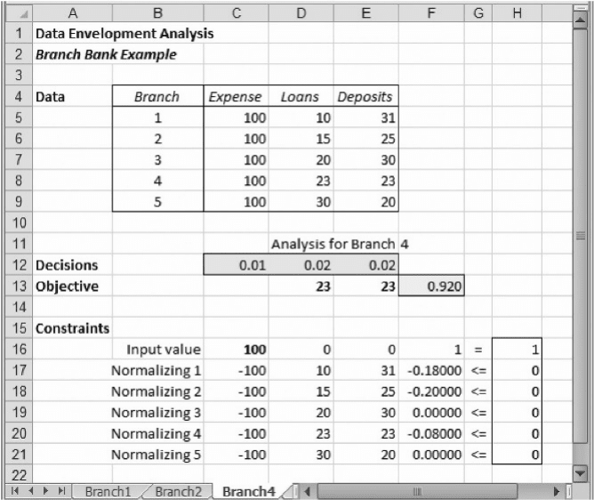
We could construct similar spreadsheet models for the analyses of Branches 3, 4,

and 5 following the same format. However, much of the content on those worksheets

would be identical, so a more efﬁcient approach makes sense. In Figure 5.5, we show a

single spreadsheet model that handles the analysis for all ﬁve branches. As before, the

array in rows 4– 9 contains the problem data. Cell F11 contains the branch number for

the DMU under analysis. Based on this choice, two adjustments occur in the linear

programming model. First, the outputs for the branch being analyzed must be selected

for use in the objective function, in cells D13:E13. Second, the inputs for the branch

being analyzed must be selected for use in the EQ constraint, in cell C16. These selec-

tions are highlighted in bold in Figure 5.5. The INDEX function uses the branch

number in cell F11 to draw the objective function coefﬁcients from the data array

and reproduce them in cells D13:E13. It also draws the input value from the data

array and reproduces it in cell C16. The three cells in bold format change when a differ-

ent selection appears in cell F11.

Figure 5.5. Model for any branch in Example 5.2.

186 Chapter 5 Linear Programming: Data Envelopment Analysis

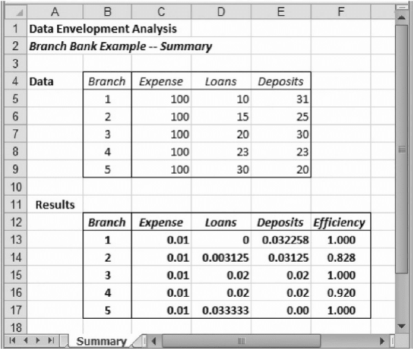
We want to solve the model in Figure 5.5 several times, once for each DMU.

To do so, we vary the contents of cell F11 from 1 to 5. Since each solution requires

a reuse of the worksheet, we save the essential results in some other place before

switching to a new DMU. In particular, we save the weights and the value of the objec-

tive function. Figure 5.6 shows a worksheet containing a summary of the ﬁve optim-

izations for the ﬁve-branch example (one from each choice of cell F11 in Figure 5.5).

The original data are reproduced in rows 4–9, and the optimal decision variables and

efﬁciencies appear in rows 12–17. This summary can be generated automatically with

the parameter analysis capability described in Chapter 4.

As we can see in Figure 5.6, there are three efﬁcient branches in our example:

Branches 1, 3, and 5. Branches 2 and 4 are inefﬁcient, with efﬁciencies of 82.8 percent

and 92 percent, respectively. The numerical results agree with the graphical model.

Thus, we have developed a spreadsheet prototype that implements the DEA approach.

Later, we build on this set of results and use the spreadsheet model to compute

additional information pertinent to the analysis.

Before proceeding, it is important to note that Example 5.2 remains somewhat

specialized. It has only one input dimension, and all the DMUs have identical input

levels. The example has only two output dimensions, but by taking the inputs to be

identical and by taking the outputs as two dimensional, we can depict the solution

graphically, as in Figures 5.1 and 5.2. As mentioned earlier, if the inputs were different

for all the DMUs, we would not have been able to convey the analysis graphically.

However, the spreadsheet model, in the same form as Figures 5.5 and 5.6, accommo-

dates the more general problem without difﬁculty.

BOX 5.1

Excel Mini-Lesson: The INDEX Function

The INDEX function in Excel ﬁnds a value in a rectangular array according to the row

number and column number of its location. The basic form of the function, as we use it

for DEA models, is the following:

INDEX(Array,Row,Column)

†

Array references a rectangular array.

†

Row speciﬁes a row number in the array.

†

Column speciﬁes a column number in the array.

In the example of Figure 5.5, suppose Array ¼ C5:E9, Row ¼ F11, and Column ¼ 2.

When cell F11 contains the number 4, the function

INDEX(C5:E9,F11,2) would

ﬁnd the element in the fourth row and second column of the array in cells C5:E9. In this

case, the function returns the Loans output value for Branch 4, or 23. This calculation

would be suitable for cell D13.

When we work with a one-column array, we can omit the Column argument in the

INDEX function. Thus, in the worksheet, we can also use the function

INDEX(D$5:D$9,$F$11) for cell D13 and then copy that formula into cell E13.

5.3. A Spreadsheet Model for DEA

187

5.4. INDEXING

Quantitative measures of performance are not always absolute ﬁgures. Often, it is more

meaningful and more convenient to measure performance in relative terms. To create

indexed data, we assign the best value on a single input or output dimension an index

of 100, and other values are assigned the ratio of their value to the best value. In effect,

all performance values are expressed in percentages, relative to the best performance

observed.

The use of indexed data does not present difﬁculties for DEA. In fact, the DEA

calculations are, perhaps, more intuitive when based on indexed data because the

result tends to be optimal weights of approximately the same order of magnitude,

which may not be the case without indexing.

To illustrate how indexing works, we return to Example 5.2. When we scan the

loan values for the various branches, the highest output in the comparison comes

from Branch 5, with an output of 30. If we treat a level of 30 as the base, we can express

the loan values for each of the other branches as a percentage of Branch 5 output.

Table 5.1 summarizes the scaled values that result, for both loans and deposits.

Suppose we perform the linear programming analysis using the indexed values

instead of the original, raw data. How does the analysis change? Figure 5.7, which

Figure 5.6. Summary of the analysis for Example 5.2.

188 Chapter 5 Linear Programming: Data Envelopment Analysis

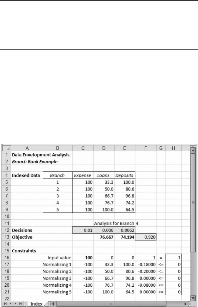
shows the analysis of Branch 4 using indexed values, conveys the main point. The

value of the objective function remains unchanged (at 92 percent in this case), even

though the values of the decision variables are different from those in the original

model (compare Figure 5.5). This example shows that the efﬁciency calculation is

robust in the sense that it depends only on the relative magnitudes of the output

levels, and these can be scaled for convenience without altering the efﬁciency

values produced by the analysis.

Within each of the output dimensions being evaluated, only relative values matter,

so it is always possible to use raw data even when the dimensions are quite different. In

Example 5.2, the sizes of loans and deposits are of roughly the same magnitude—tens

Table 5.1. Scaled Values from Example 5.2

DMU Loans Index Deposits Index

Branch 1 10 33.3 31 100.0

Branch 2 15 50.0 25 80.6

Branch 3 20 66.7 30 96.8

Branch 4 23 76.7 23 74.2

Branch 5 30 100.0 20 64.5

Figure 5.7. Analysis of Branch 4 in Example 5.2, with indexing.

5.4. Indexing 189

of millions of dollars. Suppose we had used another dimension of performance, cal-

culated as the nondefault rate on commercial and residential mortgages. For this

measure, the given data might be proportions no larger than one, but it will not be a

problem to mix such data with numbers in the tens of millions, because it is only rela-

tive levels, within a performance dimension, that really matter in DEA. As a result, we

do not have to worry about scaling the data. Nevertheless, it is sometimes advan-

tageous to use indexing because it leads to some comparability in the weights selected

by the optimization model.

5.5. FINDING REFERENCE SETS AND HCUs

We identify an efﬁcient DMU by solving the linear program and ﬁnding a value of

1 for the objective function. By contrast, an optimal value less than 1 signiﬁes that

the DMU is inefﬁcient. The ﬁrst main result in DEA is classifying the various

DMUs as either efﬁcient or inefﬁcient. For the efﬁcient DMUs, there may not be

much more to say. As we shall see later, advanced variations of the analysis can dis-

criminate among the efﬁcient DMUs. Initially, however, these are not analyzed

further. Instead, attention focuses on the inefﬁcient DMUs. If we solve a version of

the linear program and discover that a DMU is inefﬁcient, the analysis proceeds by

identifying the corresponding reference set and describing the associated HCU. In

order to carry out this part of the analysis, we can draw on the shadow price infor-

mation in the Sensitivity Report.

To illustrate how the analysis proceeds, we move next to an example with multiple

inputs and multiple outputs. The simplest such case would be a two-input, two-output

structure, as in the example of evaluating a chain of nursing homes.

EXAMPLE 5.3

Hope Valley Health Care Association

The Hope Valley Health Care Association owns and operates six nursing homes in adjoining

states. An evaluation of their efﬁciency has been undertaken, using two inputs and two outputs.

The inputs are stafﬁng labor (measured in average hours per day) and the cost of supplies

(in thousands of dollars per day). The outputs are the number of patient-days reimbursed

by third-party sources and the number of patient-days reimbursed privately. A summary of

performance data is shown in the table below.

Staff hours Supplies Reimbursed Privately paid

DMU per day per day patient days patient days

Facility 1 150 0.2 14,000 3500

Facility 2 400 0.7 14,000 21,000

Facility 3 320 1.2 42,000 10,500

Facility 4 520 2.0 28,000 42,000

Facility 5 350 1.2 19,000 25,000

Facility 6 320 0.7 14,000 15,000

190 Chapter 5 Linear Programming: Data Envelopment Analysis

A spreadsheet model for the analysis of the six DMUs is shown in Figure 5.8, which

displays the speciﬁc analysis for Facility 5. In a full set of six optimization runs for this

model, we ﬁnd that the ﬁrst four units are all efﬁcient, while Facilities 5 and 6 are inef-

ﬁcient. The efﬁciencies are summarized in cells G6:G11.

Next, we illustrate the further analysis of Facility 5. The ﬁrst step is to re-run

Solver for Facility 5 and obtain the Sensitivity Report, which is shown with some

reformatting in Figure 5.9. The information we need can be found in the

Constraints section of the Sensitivity Report, in the rows corresponding to the normal-

izing constraints of the original model, which have right-hand-side constants of zero.

The speciﬁc values we seek are the shadow prices corresponding to the six normaliz-

ing constraints, as highlighted in Figure 5.9.

To proceed, we copy the shadow prices for the normalizing constraints and paste

them into column J of the spreadsheet, so that they match up with the corresponding

constraint rows, as shown in Figure 5.8. The next step is to identify which shadow

prices are positive; the DMUs corresponding to those make up the reference set. In

Figure 5.8, we can observe that the shadow prices are positive in normalizing con-

straints corresponding to Facilities 1, 2, and 4. This means that Facilities 1, 2, and 4

form the reference set for Facility 5. The results are summarized as follows.

Shadow Reference

DMU price set

Facility 1 0.2000 Yes

Facility 2 0.0805 Yes

Facility 3 0.0000

Facility 4 0.5383 Yes

Facility 5 0.0000

Facility 6 0.0000

Having identiﬁed the reference set for Facility 5, we next construct a HCU. In

cells C26:F26 we lay out a row resembling the original row of data for Facility 5.

The entry in cell C26 is calculated as the SUMPRODUCT of the shadow prices

and the six values of the ﬁrst input (staff hours) from the array of input data. This cal-

culation yields the value 342.125, as shown below. This number represents the staff

hours of the HCU.

Staff hours Shadow

DMU per day price

Facility 1 150 0.2000

Facility 2 400 0.0805

Facility 3 320 0.0000

Facility 4 520 0.5383

Facility 5 350 0.0000

Facility 6 320 0.0000 SUMPRODUCT ¼ 342.125

5.5. Finding Reference Sets and HCUs

191

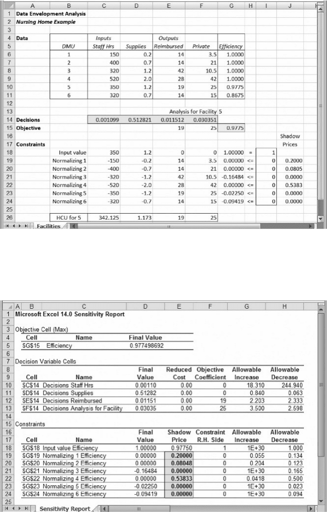
Figure 5.8. Analysis for Facility 5 in Example 5.3.

Figure 5.9. Sensitivity report for Facility 5 in Example 5.3.

192 Chapter 5 Linear Programming: Data Envelopment Analysis

The speciﬁc formula in cell C26 is ¼ SUMPRODUCT($J$19:$J$24,C6:C11).

Next, this calculation is copied to cells D26:F26, using absolute addresses for the

shadow prices in column J, as shown in Figure 5.8. The resulting numbers provide

the description of an HCU for Facility 5.

0:2000 (Facility 1 Data) ¼ 0:2000 (150 0:20 14 3:5)

0:0805 (Facility 2 Data) ¼ 0:0805 (400 0:70 14 21:0)

0:5383 (Facility 4 Data) ¼ 0:5383 (520 2:00 28 42:0)

HCU Data ¼ (342 1:17 19 25:0)

In particular, the outputs of the comparison unit, which are (19, 25), match the outputs

of Facility 5 precisely. However, the inputs (342.125, 1.173) are slightly smaller than

the inputs of Facility 5. In other words, the comparison unit achieves the same outputs

as Facility 5, but with lower input levels. By its construction, the comparison unit has

inputs and outputs that are weighted averages of those for the facilities in the reference

set. Thus, a weighted combination of Facilities 1, 2, and 4 provides a target for Facility

5 to emulate.

The analysis of Example 5.3 shows how the shadow prices can be used as weight-

ing factors to construct the HCU. In general, the comparison unit has outputs that are at

least as large as the outputs of the inefﬁcient unit being analyzed and inputs that are no

larger than the inputs of the unit being analyzed. In this case, the actual inputs for

Facility 5 are staff hours of 350 and a supply level of 1.2. The analysis suggests

that efﬁcient performance, as exempliﬁed by Facilities 1, 2, and 4, would allow

Facility 5 to produce the same outputs with inputs of only 342.125 staff hours and

a supplies level of 1.173.

How could Facility 5 achieve these efﬁciencies? DEA does not tell us. It merely

suggests that Facilities 1, 2, and 4 would be reasonable benchmarking targets for

Facility 5. Then, by studying differences in technology, procedures, and management,

Facility 5 might be able to identify and implement changes that could lead it to

improved performance.

In Example 5.3, Facilities 1–4 are all efﬁcient, but only Facilities 1, 2, and 4 form

the reference set for Facility 5. An exploration of the analysis for Facility 6 leads to a

similar conclusion: Its reference set also consists of Facilities 1, 2, and 4. Although

Facility 3 is efﬁcient, it does not appear in any reference sets. Evidently, it is not a

facility that Facility 5 or 6 should try to emulate. We might guess that this is the

case because its output mix is quite different.

5.6. ASSUMPTIONS AND LIMITATIONS OF DEA

Although we have relied on the term “efﬁcient,” it would be more appropriate to use

the term relatively efﬁcient—that is, the productivity of a DMU is evaluated relative to

the other units in the set being analyzed. DEA identiﬁes what we might call “best prac-

tice” within a given population. However, that does not necessarily mean that the

5.6. Assumptions and Limitations of DEA 193

efﬁcient units compete well with DMUs outside the population. Thus, we have to resist

the temptation to make inferences beyond the population under study.

As mentioned earlier, DEA works well when there is some ambiguity about the

relative value of outputs. No a priori price or other judgment about the relative value

of the outputs is needed. Because prices are not given, it should not be obvious

what output mix would be best. (This applies to inputs as well.) DEA performs its

evaluation by assuming weights that are as favorable as possible to the DMU being

evaluated. However, DEA may not be very useful in a situation where a distinct hier-

archy of strategic goals exists, especially if one goal strongly inﬂuences performance.

Some applications of DEA have run into complaints that the output measures may

be inﬂuenced by factors that managers cannot control. In response, variations of the

DEA model have been developed that can accommodate uncontrollable factors.

Such a factor can be added by simply including it in the model; there is no need to

specify any of its structural relationships or parameters. Thus, a factor that is neither

an economic resource nor a product, but is instead an attribute of the environment,

can easily be included. An example might be the convenience of a location for a

branch bank, which could be treated as an input.

One of the technical criticisms often raised about DEA relates to the use of com-

pletely arbitrary weights. In particular, the basic DEA model allows weights of zero on

any of the outputs. (Refer to Figure 5.3 as an illustration.) A zero-valued weight in the

optimal solution means that the corresponding input or output has been discarded in

the evaluation. In other words, it is possible for the analysis to completely avoid a

dimension on which the DMU happens to be relatively unproductive. This may

sound unfair, especially since the inputs and outputs are usually selected for their stra-

tegic importance, but it is consistent with the goal of ﬁnding weights that place the

DMU in the best possible light. In response, some analysts suggest imposing a

lower bound on each of the weights, ensuring that each output dimension receives

at least some weight in the overall evaluation. Choosing a suitable lower bound is dif-

ﬁcult, however, because of the ﬂexibility available in scaling performance data.

(Recall the discussion of indexed values earlier.) A more uniform approach is to

impose a lower bound on the product of performance measure and weight. For any

input dimension, the product of input value and weight is sometimes called the virtual

input on that dimension. Similarly, for any output dimension, the product of output

value and weight is sometimes called the virtual output. The virtual outputs are the

components of the efﬁciency measure, and we can easily require that each component

account for at least some minimal portion of the efﬁciency, such as 10 percent. In the

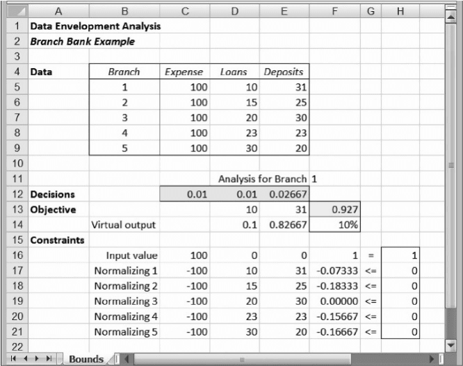
analysis of Branch 1 (see Figure 5.10), we can compute the virtual outputs for each

performance dimension in cells D14 and E14. Then, we add constraints forcing

these values to be at least 10 percent (as speciﬁed in cell F14). With these lower

bounds added, it is not possible to place all the weight on just one dimension. As

shown in Figure 5.10, the imposition of a 10 percent lower bound for the contribution

from each dimension reduces the efﬁciency rating for Branch 1 to 92.7 percent

when the model is optimized. As the example illustrates, when we impose additional

requirements, we may turn efﬁcient DMUs into inefﬁcient ones.

A related criticism is that the weight may be positive but still quite small on

an output dimension that is known to be strategically important. In this situation, it

194

Chapter 5 Linear Programming: Data Envelopment Analysis

is possible to add a constraint to the model that will force the virtual output of one

important measure to be greater than the virtual output other measures. These kinds

of additional constraints may improve the logic, but they sacriﬁce transparency in

the model.

Another technical criticism relates to the fact that a DEA evaluation often pro-

duces a number of efﬁcient DMUs, and it would be satisfying to have a tie-breaking

mechanism for distinguishing among the efﬁcient units. One way to break ties is to

omit the normalizing constraint for the kth DMU when it is the subject of evaluation.

When we do so, we tend to get some efﬁciencies above 1.0, and we are much less

likely to get ties in the performance metric. Another response is more complicated

but perhaps more equitable. The evaluation of the kth DMU produces a set of optimal

weights that are, presumably, as favorable as possible to unit k. Suppose we call these

“price set k.” When we evaluate DMU k, we compute the value of its outputs under

each of the price sets (price set 1, price set 2, etc.). Then we average the output

values obtained under the various price sets and rank the DMUs based on their average

values over all price sets. The average value on which the DMUs are ranked is called

the cross-efﬁciency. This method makes ties less likely but involves more

computation.

Although we started with a small one-input/one-output example and then moved

on to larger examples, it does not follow that a DEA model should be built with as

many inputs and outputs as possible. In fact, there is a good reason to limit the

Figure 5.10. Analysis of Branch 1 with lower bounds.

5.6. Assumptions and Limitations of DEA 195