Bernatz R. Fourier Series and Numerical Methods for Partial Differential Equations

Подождите немного. Документ загружается.

142 HEAT TRANSFER IN 2D AND 3D

The orthonormality of the eigenfunctions X

(x) and Y

(y) gives

rC pd

(x)Ym(y)Xr(x)Ys(y)dydx = { J

if n φ r or m ^ s

if n = r and m = s

(6.17)

Therefore, if coefficients .A

exist such that Equation (6.16) is true, then

pc pd

= I X

(x)Ym{y)f(x,y)dydx (6.18)

Jo Jo

6.1.1 Example: Homogeneous IBVP

The solution procedure outlined in the Section 6.1 is used to solve the following

homogeneous IBVP,in two dimensions:

( u

(x,y,t) = k[u

(x,y,t) +u

{x,y,t)]

u(x,y,0) = f(x,y)

IBVP<

(PDE)

(IC)

(x, 0, t) = 0 0 < x < c (BC1)

u\c, y,t) = 0 0 < y < d (BC2)

u\x, d,t) = 0 0<x<c (BC3)

I w(0,2/,i) = 0 0<y<d (BC4)

(6.19)

Note the temperature is held at the constant value of zero at all boundaries except

that for y = 0, where the boundary is insulated. The problem is said to have

mixed boundary conditions because two types of boundary conditions (Dirichlet and

Neumann in this case) are specified.

The Dirichlet-Dirichlet boundary conditions on the function X mean the eigen-

values are

, 2

a„

and the eigenfunctions are

(T)'

Xn(x)

n = 1,2,3,...

- sin a

The Neumann-Dirichlet boundary conditions for the Sturm-Liouville problem in

Y result in eigenvalues of

2 i'(2m

—

1)π

/r =

with associated eigenfunctions

—

1,2,3,...

Ym(y) = \ -cosß

SEMIHOMOGENEOUS 2D IBVP 143

Suppose the initial temperature distribution is given by

il 0.8 < x < 1.2 and 0.3 < y < 0.7

ffay) = \ " " "

t 0 otherwise

If k = 0.1, c = 2 and d = 1 the temperature u(x, y, t) is given by

u(x,y,t) =

Σ Σ

™™

(ψ)

-((

- - D^)e-°

[

(¥)

^"^l*

n—1 ra=l

where

Aim = / / /(a:,

2/)

sin ( —— j y/2 sin((2m - l)ny)dydx

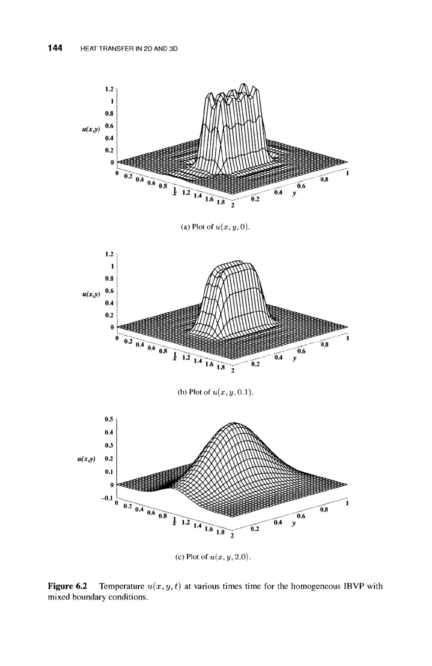
The temperature u(x,y,t) for various times £ is plotted in Figure 6.2. The

graph of u(x, y, 0) is shown in Figure 6.2(a), which shows how the double Fourier

series matches the discontinuous initial temperature f(x,y) distribution within the

rectangular region. The Fourier representation in this example is constructed with m

and n = 20. It has some difficulty at the "edges" of the nonzero section of /(x, y).

The temperature distribution appears much smoother for time t — 0.1, as shown in

Figure 6.2(b). The temperature is fixed at zero at three of the four boundaries, and

insulated where y = 0, so as time increases, the overall temperature of the material

will decrease to zero at all locations, including the insulated boundary. However, the

temperature at the points on this boundary remains positive as indicated in Figure

6.2(c). Note that the vertical scale (the temperature) is less in Figure 6.2(c) so that

the Neumann condition may be more clearly seen.

6.2 SEMIHOMOGENEOUS 2D IBVP

A general semihomogeneous 2D IBVP is outlined in IBVP (6.20). The nonhomoge-

neous nature of the IBVP is contained in the PDE where the internal heat source or

sink function q(x, y, i) is included.

ut = k [u

+ u

] + q(x, y, t) (PDE)

U(X,Î/,0) = /(X,Î/) (IC)

aiu(x,0,t)+a

(x,0,t) = 0 0<x<c (BC1)

(

)

IBVP<

hu(c,y,t) + b

(c,y,t) =0 0 < y < d (BC2)

c\u{x,d,

t) + C2U

(x, d, t) = 0 0<x<c (BC3)

diu(0,í/,í) +d

Mx(0,y,i) = 0 0 < y < d (BC4)

The method for solving the semihomogeneous IBVP in 2D is like that for the ID

case where variation of parameter methods were used. For the 2D, case we begin by

assuming a solution of the form

OO OO

u(x, y, t) = Σ Σ A

m{t)X

{x)Ym{y)e-

k(al+ß

(6.21)

n=0 m=0

144 HEAT TRANSFER IN 2D AND 3D

u(x,y)

1.2 i

0.8 \

0.6

0.4

0.2

0.6

0.4 y

(a)Plotofu(rr,y,0).

u(x,y)

(b) Plot ofu(x,y, 0.1).

Figure 6.2 Temperature w(x, y, í) at various times time for the homogeneous IBVP with

mixed boundary conditions.

SEMIHOMOGENEOUS 2D IBVP

145

where the double Fourier coefficients A

nrn

(t) are time-dependent parameters to be

determined. As in the ID case, the actual form of u(x,y,t) used in the solution

process is

u(x,tf,

= Σ Σ

nrn

{t)X

{x)Y

(y) (6.22)

n=0 ra=0

where

The heat source or sink term q(x, y, t) will be represented by the double Fourier

series

q(x, y, t) = Σ Σ

Qnm(t)Xn(x)Ym(y)

(6.23)

n=0 m=0

where

Qnm(t)

= /

q(x,y,t)X

(x)Y

(y)dydx (6.24)

Substituting the expression for u{x, y, t) in Equation (6.22) and the expression for

q(x, y, t) in Equation (6.23) into the PDE of IBVP (6.20) gives

oo oo oo

(t)X

(x)Y

(y)

ΣΣ-1;[αΙ+

]

(t)X

(x)Y

(y)

n=0 m=0

Σ Σ

Qnm(t)Xn(x)Ym(y) (6.25)

n=0m=0 n=0m=0

n=0 m=0

V (~\

α«Λ

V"f„\

—

—fß

where the facts that X'¿(x)

-ο%Χ

(χ) and

Y^(y) =

-ßm

m(y) are used to

write the derivatives of

and

in terms of

and

respectively.

Assuming equality in the double series expressions implies equality of the corre-

sponding individual terms implies

(t)

+ k

+ ßl]

(t)

(6.26)

for each nra-term,

n =

0,1,2,... and m

0,1,2, Equation (6.26) is

first-

order, linear, nonhomogeneous differential equation for each nm-pair. The solution

to a given nm-equation is found through the use of an integrating factor

so that

(t)

= e-

K+Ä)'

Qnro(T)e

*(<*+/£)T

Cmne

-k(

fi'

(62Ί)

Using the initial condition

(0)

(0)e-

^+^°

—

Γ /

/(^,2/)^n(^)^m(2/)d^x (6.28)

146 HEAT TRANSFER IN 2D AND 3D

it follows that

re pd

/ f(x,y)X

(x)Ym(y)dydx

Jo Jo

so that the formula for B

(t) is

(t)

= e-

^y\fQ

{r)e

^>dr

VJo

+ f(x,y)Xn(x)Ym(y)dydx\

Jo Jo

(6.29)

where

rC pd

Jo Jo

Qnm{t)= / q(x

y,t)X

(x)Y

(y)dydx

IBVP<

This solution procedure is used in the following example of

internal heat source

and sink.

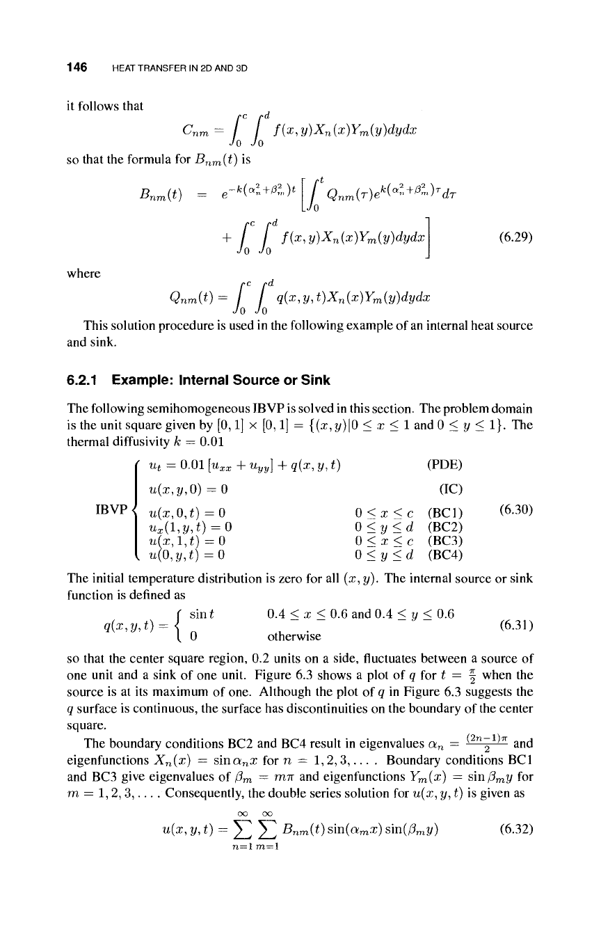
6.2.1 Example: Internal Source or Sink

The following semihomogeneous IBVP is solved in this section. The problem domain

is the unit square given by [0,1] x [0,1] = {(x, y)\0 < x < 1 and 0 < y < 1}. The

thermal diffusivity k

—

0.01

= 0.01 [u

Uyy)

+ q(x, y, t) (PDE)

u(x,y,0)=0 (IC)

w(x,0,í)

0 0<x<c

(BC1)

(6.30)

Mx(l,2/,t)

0<y<d (BC2)

u{x,

0<x<c (BC3)

i¿(0,2/,t)

0<y <d (BC4)

The initial temperature distribution is zero for all (x, y). The internal source or sink

function is defined as

f sint 0.4 < x < 0.6 and 0.4 < y < 0.6

q(x,V,t) = {

^ " . " - - (6.31)

t 0 otherwise

so that the center square region, 0.2 units on a side, fluctuates between a source of

one unit and a sink of one unit. Figure 6.3 shows a plot of q for t = | when the

source is at its maximum of one. Although the plot of q in Figure 6.3 suggests the

q surface is continuous, the surface has discontinuities on the boundary of the center

square.

The boundary conditions BC2 and BC4 result in eigenvalues a

= ^

~ ^ and

eigenfunctions X

(x) = sina

x for n — 1,2,3,... . Boundary conditions BC1

and BC3 give eigenvalues of

= πιπ and eigenfunctions Y

(x) — smß

y for

m = 1,2,3,... . Consequently, the double series solution for u(x,

?/,

t) is given as

oo oo

u(x,

2/,

i) = 5Z Σ

nm(t) sin(a

x) sin(ß

y) (6.32)

NONHOMOGENEOUS 2D IBVP 147

q(*,y)

Figure 6.3 Plot of q(x, y, t) for t = f.

where the time-dependent coefficients B

(t) are given by

¿W¿) = e-

001

^^ [| (j j q(x,y,T)8m(a

x)sm(ß

y)dydx

\dT

+ / / 0 · sin(a;

x) sm(ß

y)dydx

(6.33)

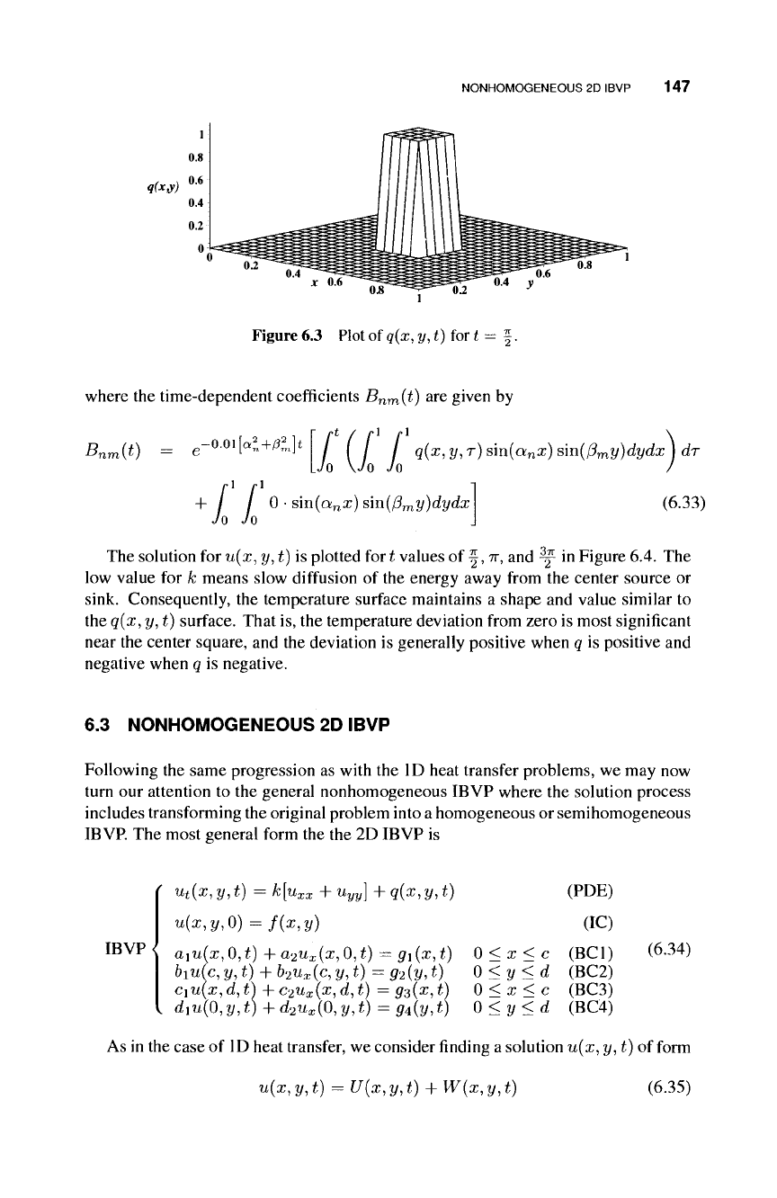
The solution for u(x, y, t) is plotted for t values of Ç, π, and ^y in Figure 6.4. The

low value for

means slow diffusion of the energy away from the center source or

sink. Consequently, the temperature surface maintains a shape and value similar to

the q(x, y, t) surface. That is, the temperature deviation from zero is most significant

near the center square, and the deviation is generally positive when q is positive and

negative when q is negative.

6.3 NONHOMOGENEOUS 2D IBVP

Following the same progression as with the ID heat transfer problems, we may now

turn our attention to the general nonhomogeneous IBVP where the solution process

includes transforming the original problem into

homogeneous or semihomogeneous

IBVP.

The most general form the the 2D IBVP is

ut(x, y, t) = k[u

Uyy)

+ q(x, y, t) (PDE)

U(X,Î/,0) = /(X,Î/) (IC)

u(x,0,t)+a

(x,0,t) = g

(x,t) 0<x<c (BC1)

(

)

biu(c, y, t) 4- b

(c, y, t) = g

{y, t) 0 < y < d (BC2)

c\u(x,d,

t) 4- C2U

(x,d, t)

—

gs(x,t) 0<x<c (BC3)

u{0,y,t)+d

(0,y,t)=g

(y,t) 0<y<d (BC4)

As in the case of ID heat transfer, we consider finding a solution u(x, y, t) of form

IBVP^

u(x, y, t) = U(x, y, t) + W(x, y, t)

(6.35)

148 HEAT TRANSFER IN 2D AND 3D

(a) Temperature at t = Ç

(b) Temperature at t

—

Figure 6.4 Temperature at various times for the semihomogeneous IBVP with mixed

boundary conditions.

NONHOMOGENEOUS 2D IBVP 149

where U will be determined by separation of variables and Fourier series methods on a

semihomogeneous IBVP, and W satisfies the nonhomogeneous boundary conditions

of IBVP (6.34). Another condition placed on W will become evident as the details

unfold below.

We begin by substituting the expression for u(x, y, t) in Equation (6.35) into the

PDE of the IBVP (6.34).

(x, y, t) + W

(x, y,t) = k [V

U(x, y, t) + V

W(x, y, t)] + q(x, y, t) (6.36)

where

V = 1

Rearranging Equation (6.37) gives

(x,y,

t) = kV

U(x, y, t) + kV

W{x, y, t) + q(x, y, t) - W

(x, y, t) (6.37)

If we require

W(x,y,t)

= 0 (6.38)

then Equation (6.37) simplifies to

(x, y, t) = kV

U(x,y, t) + q(x,y, t) - W

(x, y, t) (6.39)

which will represent the nonhomogeneous PDE of a semihomogeneous IBVP for U.

Because the IBVP for U must have homogeneous boundary conditions, it follows

that any nonhomogeneous BCs of the original IBVP (6.34) must be satisfied by the

W function. Assuming such a W exists, the following semihomogeneous IBVP

defines the function U

= kV

U + q(x,y,t)-W

(x,y,t)

t/(x,y,0) = /(x,y)-W(a;,y,0)

IBVP<

(PDE)

(IC)

aiU(x, 0, t) + a

(x, 0, t) = 0 0<x<c (BC1)

hU(c,y,t) + b

(c,y,t) =0 0 < y < d (BC2)

cit7(x, d, t) + c

(x, d, i) = 0 0<x<c (BC3)

dit/(0,

y, ¿) + d

(0, y, t) = 0 0<y<d (BC4)

(6.40)

Knowing that we can solve the IBVP (6.40) for U, the next task is determining

the function W that satisfies Equation (6.38) and the nonhomogeneous boundary

conditions of

the

original IBVP (6.34). To make this process simpler, we will assume

for the time being that the boundary functions g\ through

g±

are not time dependent.

This would imply that

W = W(x,y)

and the problem that defines

is a BVP only. That is, we are looking for a function

W(x,y),

suchthat

BVP<

W(x,y)=0

W{x,0) + a

(x,0)

W(c,y) + b

(c,y)

ciW(x, d) 4- c

(x, d

diW(0,y)+d

Ws(0,y:

0i W

92\y)

9s(x)

94{y)

0<x<c

0<y <d

0 <x<c

0< y <d

(PDE)

(BC1)

(BC2)

(BC3)

(BC4)

(6.41)

150 HEAT TRANSFER IN 2D AND 3D

The PDE in the BVP is the Laplace equation in W. Eventually, we will consider

a BVP similar to (6.41), except the PDE will be the non-homogeneous Poisson

equation

W(x,y)

= f(x,y)

Section 6.4 will focus on methods for solving various BVPs.

6.4 2D BVP: LAPLACE AND POISSON EQUATIONS

Laplace and Poisson BVPs arise in many circumstances in physics, chemistry, and

engineering. We saw in Section 6.3 that a Laplace BVP results in our method for

solving general 2D nonhomogeneous IBVPs.

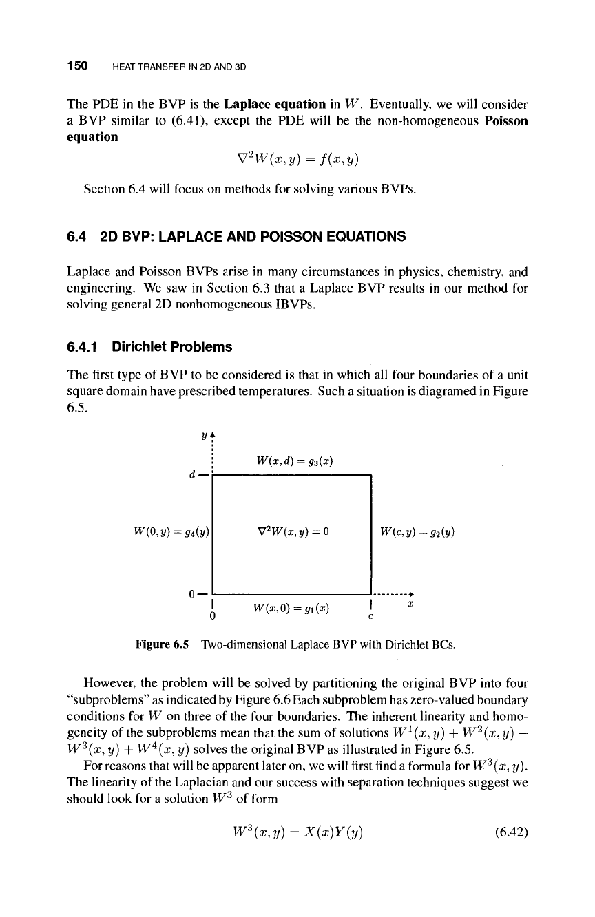
6.4.1 Dirichlet Problems

The first type of BVP to be considered is that in which all four boundaries of a unit

square domain have prescribed temperatures. Such a situation is diagramed in Figure

6.5.

w(p,v)

= 9A(y)

W(x,d)=g

(x)

W(x,y)=0

W(x,0) =

(x)

W{c,y) =g

(y)

Figure 6.5 Two-dimensional Laplace BVP with Dirichlet BCs.

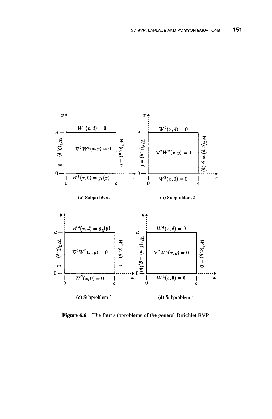
However, the problem will be solved by partitioning the original BVP into four

"subproblems" as indicated by Figure 6.6 Each subproblem has zero-valued boundary

conditions for W on three of the four boundaries. The inherent linearity and homo-

geneity of the subproblems mean that the sum of solutions W

(x^ y) + W

(x, y) +

(x, y) 4- W

(x, y) solves the original BVP as illustrated in Figure 6.5.

For reasons that will be apparent later on, we will first find a formula for W

(x, y).

The linearity of

the

Laplacian and our success with separation techniques suggest we

should look for a solution W

of form

(x,y)=X(x)Y(y)

(6.42)

2D BVP: LAPLACE AND POISSON EQUATIONS 151

(a) Subproblem 1 (b) Subproblem 2

2/f

(x,d)

= g

(y)

(x,d)

= 0

(x,y)

= 0

(x,0)

= 0

-♦►0

—

*s-~v

«Cf

W\x,y)

= 0

{x,0)

= 0

*».

Figure 6.6 The four subproblems of the general Dirichlet BVP.