Bernatz R. Fourier Series and Numerical Methods for Partial Differential Equations

Подождите немного. Документ загружается.

This Page Intentionally Left Blank

CHAPTER 5

HEAT TRANSFER IN 1D

The techniques of separation of variables and Fourier series are used to solve a

variety of ID heat transfer problems in this chapter. The homogeneous IBVP is

solved initially. Then the method of variation of parameters is used to solve IBVPs

for the case of a nonhomogeneous PDE with homogeneous boundary conditions.

This type of IBVP is referred to as the semihomogeneous problem. Once this

solution procedure is in place, the general nonhomogeneous problem, where one

or both boundary conditions is nonhomogeneous, is solved by transforming the

nonhomogeneous IBVP to a semihomogeneous problem.

5.1 HOMOGENEOUS IBVP

The development of a solution process for a general ID IBVP begins by considering

the simpler homogeneous version of an IBVP. The general form of the problem is

Fourier Series and Numerical Methods for Partial Differential Equations, 113

First Edition. By Richard Bernatz

114 HEAT TRANSFER IN 1D

outlined as

IBVP<

= ku

(x,t), 0 < x < c (PDE)

u(x

0) = /(x)

aiu(0, t) + a2U

(0, t)

b\u(c,t)

+ b2U

(c,t) -

(IC)

(BC1)

(BC2)

(5.1)

The PDE and both BCs are homogeneous. In the case of the BCs, a\ or

Ü2

must

nonzero in

BC1,

and b\ or

must be nonzero in

BC2.

The IB VP define by Equations

(5.1) is stated generally so that it includes the possibility of any of

the

three boundary

condition types at either of the boundary locations. The case of insulated ends

(Neumann-type conditions at both x = 0 and x

—

c) is solved next example.

5.1.1 Example: Insulated Ends

Recall the initial example of the method of separation of variables presented in

Section 1.8 was for the ID heat transfer problem with Dirichlet boundary conditions

(boundary conditions of the first type). The first example in this chapter is for the

case of insulated boundaries at x = 0 and x = c (Neumann boundary conditions or

boundary conditions of the third type).

Consider the IBVP

IBVP<

—

\x,t),

u(x,0) = f(x)

Ό,ί)

= 0

c,t) =0

0 < x < c (PDE)

(IC)

(BC1)

(BC2)

(5.2)

corresponding to heat transfer in an infinite slab bounded by the planes x = 0 and

x = c or a thin metal rod lying parallel to the x-axis with ends at x = 0 and x — c.

The boundary conditions specified above imply the slab and rod are insulated at

x = 0 and x

—

c. The objective is to find a formula for u(x,t) that satisfies the IBVP.

Using the method of separation of variables, the solution for u(x, t) is assumed to

be of the form u(x, t)

—

X(x)T(t). Substituting for u and its derivatives in the PDE

of IBVP 5.2 gives

X(x)T'(t) = kX"{x)T{t)

Dividing both sides of this equation by X(x)T(t) results in

T'(t) _ X"{x)

kT(t) ~ X(x)

Because the left-hand side of the last equation is a function of t while the right-hand

side is a function of x, it follows that both sides of the equation may be, at most, a

constant. Let — λ be the separation constant. Then, the equation given above may be

separated into two ODEs:

X"{x)

+ XX(x) = 0 (5.3)

T'{t) + XkT(t) = 0

(5.4)

HOMOGENEOUS IBVP 115

The boundary conditions of IBVP 5.2 applied to the assumed form of u(x, t) gives

(0,t) = 0 => X'(0)T(t) =0=> X'(0) = 0

and

(c,t) = 0 => X'(c)T(t) = 0 => X'(c) = 0

The requirements of X'(0) = X'(c) = 0 are made to ensure a nontrivial solution for

T(£).

That is, we do not want to specify T(t) = 0 in either case.

Combining Equation (5.3) with the boundary conditions on X gives

X"{x)

+ XX (x) = 0 (5.5)

X'(0)

= 0 X'(c) = 0 (5.6)

which is the Regular Sturm-Liouville example presented in Section

3.4.1.

The

resulting eigenvalues for this problem are λ

= (ηπ)

for n = 0,1,2,... with

corresponding eigenfunctions X(0) = 1 and X

(x) = cos (

^), n

—

1,2,3,....

Now that the eigenvalues have been determined through the Regular Sturm-

Liouville problem, the ODE for T given by (5.4) becomes

T'{t) + k(nw)

T{t) = 0 (5.7)

for n = 0,1,2,... . For n

0, Equation (5.7) becomes T'(t) = 0 so that the general

solution is a constant multiple of To(t) = 1. For n = 1,2,3,..., the resulting

first-order, linear, homogeneous ODE given by Equation 5.7 has a general solution

that is a constant multiple of the function

(t) =

fc(mr)2t

Combining the solutions for X and T results in solutions for u(x, t) of the form

uo(x,t) = X

(x)T

(t) = 1

and

(χ, t) = Xn(x)T

(t) = cos(nnt)e-

k{n7r)H

, n = 1,2, 3,...

Applying the generalized principle of superposition, we know the expression

u{x,t) = ^ + Y

cos(nnx)e-

k(n

is a function that satisfies the homogeneous PDE and both homogeneous boundary

conditions of Equation (5.2).

The solution process will be complete once the nonhomogeneous initial condition

is satisfied. To that end, we require

u(x, 0) = f(x) =» ^ + Σ

cos(nnx)e-

kin7r)2

° = f{x)

n=l

=> -y + 5Z «n οο8(ηπχ) = /(x)

n=l

116 HEAT TRANSFER IN 1D

Given that function f(x) is piecewise smooth and defined in such a way that

(I)

„ ΛΞζ1±1ίΞ±)

for all x in

(0,1

it follows from Theorem 2.7 that the cosine series

V 2_\

n cos(n7rx) (5.8)

n=l

with

—

2 / f(x)cos(nnx)dx n

—

0,1,2,... (5.9)

will converge to f(x) for all x in (0,1). Refer to the summary comments in Section

2.13 for support of this convergence claim.

5.2 SEMIHOMOGENEOUS PDE

Suppose an infinite slab with faces at x

—

and x = c has an internal heat source given

by q(x, t). The general ID IBVP in this case is given as

IBVP<

= ku

(x,t) 4-

q(x,t),

0<x<c (PDE)

u(x,0)=/(x) (IC)

(5AQ)

u{0,t)+a

(0,t) = 0 (BCl)

t biu(c,t) + b

(c,t) = 0 (BC2)

so the PDE in this application is nonhomogeneous. Both prescribed boundary con-

ditions for the IBVP (5.10) are homogeneous. From now on, we will refer to such an

IBVP as semihomogeneous.

We know for the homogeneous case (q(x, t)

—

0) the solution will have the form

u{x,t) = Y^A

{x)e-

n=0

where a

and X

(x) are, respectively, the eigenvalues and orthonormal eigenfunc-

tions for the associated Sturm-Liouville problem determined by the values of a±,

(22,

&i, and

&2·

The eigenfunctions will be sine or cosine functions for any scenario

because of the homogeneous boundary conditions. In some instances, the index n

may begin at

"1"

instead of

"0."

The coefficients A

are determine in the usual way

using the initial condition f{x). That is,

f{x)X

(x)dx

SEMIHOMOGENEOUS PDE 117

5.2.1 Variation of Parameters

The method presented in this section for determining a solution to the nonhomo-

geneous IBVP (5.10) is based on the variation of parameters method used in the

case of nonhomogeneous ordinary differential equations.

refresh ourselves of this

method, suppose we want to solve the nonhomogeneous, linear, second-order ODE

y"(t)+ay

(t)

+ by(t) = f(t) (5.11)

where a and b are constant coefficients. Given that yi(t) and y

{t) are linearly

independent solutions of the homogeneous form of Equation (5.11), the general

solution of homogeneous ODE is

y(t) = ciyi(t) +

(t)

where the constants c\ and c

may be determined

the appropriate initial or boundary

conditions to specify a particular solution to the ODE.

The method of variation of parameters assumes a particular solution to the non-

homogeneous ODE in Equation (5.11) has the form

y(x)=c

(t)yi(t)+c

(t)y

(t)

and the functions c\ and c

are determined by requiring the form of y given above to

satisfy the original Equation (5.11). Some additional restrictions on c\ and c

may

be required to simplify the process for determining expressions for these functions.

Following a similar approach for the nonhomogeneous PDE of IBVP (5.10), we

assume the solution will be of the form

u(x,t) = J2A

(t)X

(x)e-

^, (5.12)

where X

(x) are orthonormal eigenfunctions corresponding to the eigenvalues a

Letting B

(t) = A

{t)e~

koi

, the sum shown in Equation (5.12) has the simpler

form

u(x,t) =

Y^B

(t)X

(x)

(5.13)

n=0

As with the ODE case, the objective is to find expressions for the parameters

(t),

n = 0,l,2,....

In order to determine expressions for

{t),

we begin by expressing the function

q(x, t) in terms of the orthonormal eigenfunctions X

{x)· That is,

q(x,t) =

Y^Q

(t)X

(x)

(5.14)

71=0

where

Qn(t)= [ q(x,t)X

(x)dx (5.15)

118 HEAT TRANSFER IN 1D

Now the PDE in IBVP (5.10) may be written as

(x,t) = ku

(x,t) -\-^2Q

(t)X

(x) (5.16)

n=0

Subbing for u

and u

in terms of the corresponding series forms gives

oo oo oo

Σ B'

(t)X

(x) = kJ2 -a

(t)X

(x) + Σ Qn(t)X

(x) (5.17)

n=0 n=0 n=0

Here, we are assuming the derivatives of u(x,t) [given in Equation (5.13)] with

respect to t and x (twice) of the infinite series are simply the infinite series of the

component derivatives. Additionally, because the eigenfunctions for this situation

are either sines or cosine terms, it follows that:

X;'(x) = -a

(x).

Moving the first term on the right- to the left-hand side and associating the sums

gives

oo oo

Σ [K(t)

+ ka

(t)]

{x) = Σ Q

(t)X

(x)

(5.18)

n=0 n=0

Assuming equality in the infinite series implies equality of terms for each value n

results in the ODE

(t)

+ ka

(t) = Q

(t) (5.19)

Using the initial condition of the IBVP (5.10),

u(x,0) = f(x) => ¿ B

(Q)X

(x) = f(x)

n=0

so that

Bn(0) = Í f(x)X

(x)dx

(5.20)

(5.21)

which provides an initial condition on B

(x) to go along with the first-order linear

ODE for B

(x) given in Equation (5.19).

The ODE in Equation (5.19) is solved using the integrating factor

μ{ί) = e

katt

to give

(t)

-kalt

I Qn(r)e

dT+ Γ f(x)X

(x)á

Jo Jo

j (Γ q(x,r)X

(x)dx) e

dr + Γ f(x)X

(x)dx

for the time-dependent coefficients

(t).

-katt

SEMIHOMOGENEOUS PDE 119

5.2.2 Example: Semihomogeneous IBVP

Consider the IBVP given below.

= 0.1u

(x, t) -f q{x, t), 0 < x < 1

u(x,0) = x(l

—

IBVP<

0,i

1,*'

(PDE)

(IC)

(BC1)

(BC2)

(5.22)

The boundary conditions indicate the infinite slab has insulated faces at x — 0 and

x = 1. The initial temperature distribution is f(x) =

x(l—x).

In terms of the internal

heat generation term, suppose q(x, t) is given by

the

product

#[0.45,0.55]

(#)e

, where

#[0.45,0.55] (

)

0.45 < x < 0.55

otherwise

(5.23)

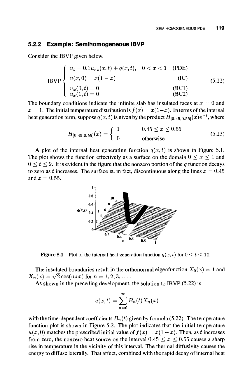
A plot of the internal heat generating function q(x,t) is shown in Figure 5.1.

The plot shows the function effectively as a surface on the domain 0 < x < 1 and

0 < t < 2. It is evident in the figure that the nonzero portion of

the

q function decays

to zero as t increases. The surface is, in fact, discontinuous along the lines x

—

0.45

and x = 0.55.

qM)

Figure 5.1 Plot of

the

internal heat generation function q(x,t) for 0 < t < 10.

The insulated boundaries result in the orthonormal eigenfunction XQ{X) — 1 and

Xn(%) =

Λ/2

cos(nnx) for n = 1,2,3,... .

As shown in the preceding development, the solution to IBVP (5.22) is

L{x,t) = Y^B

{t)X

{x)

n=0

with the time-dependent coefficients B

(t) given by formula

(5.22).

The temperature

function plot is shown in Figure 5.2. The plot indicates that the initial temperature

u(x, 0) matches the prescribed initial value of f(x) = x(l

—

x). Then, as t increases

from zero, the nonzero heat source on the interval 0.45 < x < 0.55 causes a sharp

rise in temperature in the vicinity of this interval. The thermal diffusivity causes the

energy to diffuse laterally. That affect, combined with the rapid decay of internal heat

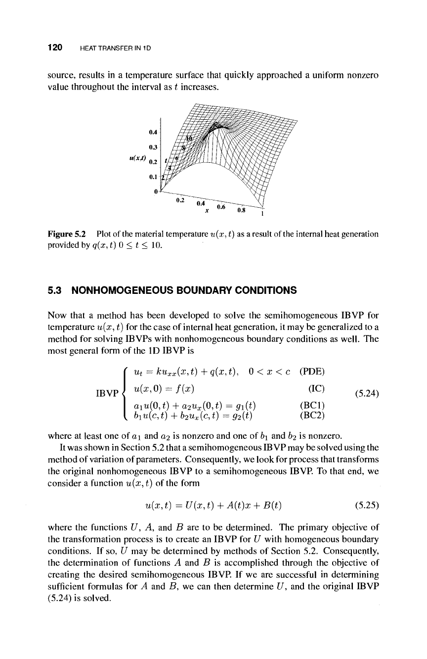
120 HEAT TRANSFER IN 1D

source, results in a temperature surface that quickly approached a uniform nonzero

value throughout the interval as t increases.

u(x¿)

Figure 5.2 Plot of the material temperature u(x, t) as

result of

the

internal heat generation

provided by q(x, t) 0 < t < 10.

5.3 NONHOMOGENEOUS BOUNDARY CONDITIONS

Now that a method has been developed to solve the semihomogeneous IBVP for

temperature i¿(x, t) for the case of internal heat generation, it may be generalized to a

method for solving IBVPs with nonhomogeneous boundary conditions as well. The

most general form of the ID IBVP is

IBVP<

—

{x, t) 4- q(x, t), 0 < x < c (PDE)

u(x,0)=f(x) (IC)

aitt(0,

t) 4- a

(0, t) = gi(t)

&iu(c, t) 4- b

(c, t) = g

(t)

(5.24)

(BC1)

(BC2)

where at least one of a\ and a

is nonzero and one of b\ and b

is nonzero.

It was shown in Section 5.2 that

semihomogeneous IBVP may be solved using the

method of variation of parameters. Consequently, we look for process that transforms

the original nonhomogeneous IBVP to a semihomogeneous IBVP. To that end, we

consider a function u(x, t) of the form

u(x, t) = U(x, t) + A(t)x 4- B(t)

(5.25)

where the functions U, A, and B are to be determined. The primary objective of

the transformation process is to create an IBVP for U with homogeneous boundary

conditions. If so, U may be determined by methods of Section 5.2. Consequently,

the determination of functions A and B is accomplished through the objective of

creating the desired semihomogeneous IBVP. If we are successful in determining

sufficient formulas for A and B, we can then determine U, and the original IBVP

(5.24) is solved.

NONHOMOGENEOUS BOUNDARY CONDITIONS 121

The process of transforming the original IBVP (5.24) to one for U with homoge-

nous boundary conditions is outlined next. We begin with the PDE.

PDE

Ut{x, t) = ku

(x, t) 4- q{x, t)

(x, t) 4- A\t)x + B'{t) = kU

(x, t) + q{x, t)

(x, t) = kU

(x, t) 4- q(x, t) - A

(t)x - B'(t)

{x,t)

= kU

(x,t) +q*(x,t)

where q*{x,t) = q{x,t) - A'(t)x -

B'(t).

Next, we find an initial condition for U.

Initial Condition

u(x,0)=f(x)

=$> U(x, 0) + A(0)x 4- J3(0) = f(x)

=> U{x, 0) = f(x) - A(0)x - B(0)

=* U(x,0) = f*(x)

where /*(x) - U(x,0) - A(0)x - B(0).

BC at x = 0

aiw(0,i) + a

(0,i) = #i(¿)

ai(C/(0,f) 4- A(i) · 0 4- B(t)) + a

(^(0,t) 4- A(f)) = ^i(t)

aiî/(0,

¿) 4- a

(0, t) + α

Α(ί) 4- a

B{t) = g

(t)

BC at x

biu(c,t) 4- b

(c,t) =

02 (¿)

=» 6i(C/(c,t) + A(t) .c + B(í)) + 62(üx(c,í) + A(í)) = <?

(¿)

=> ^[/(c, t) 4- fcC^c, t) 4- (he 4- 6

)A(t) 4- 6iB(i) = g

(t)

Requiring homogeneous BCs for U at both x = 0 and x = c results in the

following system of equations

A(t) + aiB(t) = #i(t) (5.26)

+ 6

),4(t)4-&i£(¿) = g

(t) (5.27)