Bernatz R. Fourier Series and Numerical Methods for Partial Differential Equations

Подождите немного. Документ загружается.

162 HEAT TRANSFER IN 2D AND 3D

2/f

(x,l)

= 0

-W

(0,î/) = 4(l-y)-2

W(x,y)

= 0

(x,0)

= 0

(2,y)=0

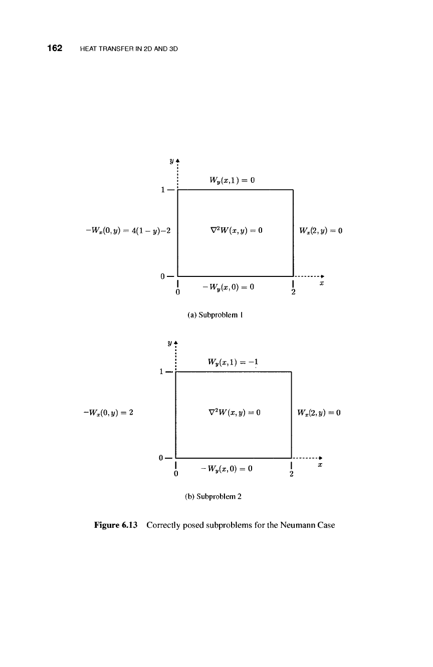
(a) Subproblem 1

2/f

(ar,l)

= -1

-W*(0,y) = 2

W{x,y)

= 0

(2,y)

= 0

¿ -Τν

(χ,0) = 0

(b) Subproblem 2

Figure 6.13 Correctly posed subproblems for the Neumann Case

BVP:

LAPLACE AND POISSON EQUATIONS 163

(x,0)=0

WÎ{xA)

E =

C =

0 + E =

1 = -1

The result of satisfying the BCs is

W\x,y)=

-x

-y

(6.95)

(6.96)

so that, as in the case of the first subproblem, we are able to determine a formula for

(x, y) up to a constant. In this case, as in the previous case, we will let F = 0.

Combining the formulas for W

(x, y) and W

(x, y) gives the nonunique solution

11 °°

W(x, y) — -x

—

2x + 2_.

n cos(nny) cosh(n7r(l

—

x)) (6.97)

n=l

with coefficients a

given by Equation (6.93).

0.5 1

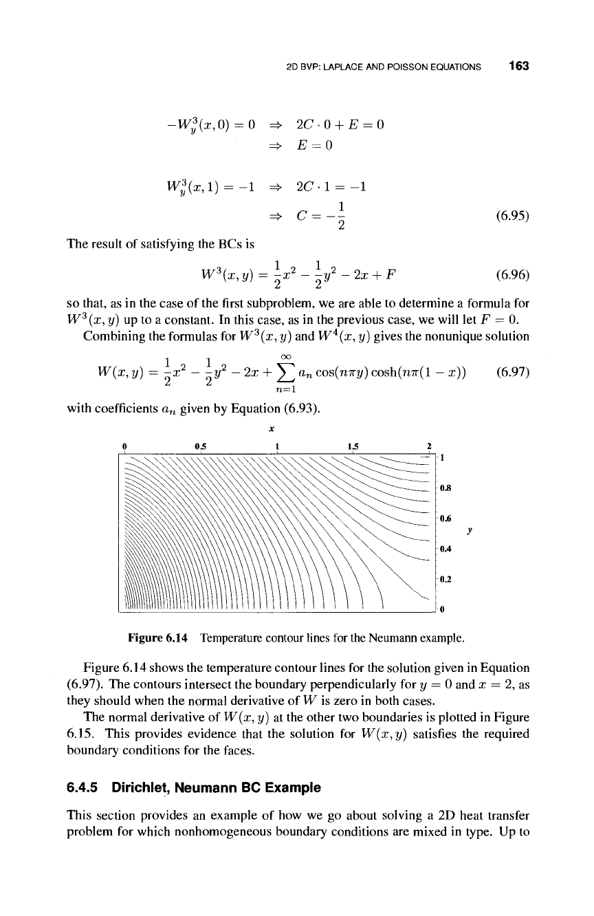
Figure 6.14 Temperature contour lines for the Neumann example.

Figure 6.14 shows the temperature contour lines for the solution given in Equation

(6.97).

The contours intersect the boundary perpendicularly for y

—

0 and x

—

2, as

they should when the normal derivative of W is zero in both cases.

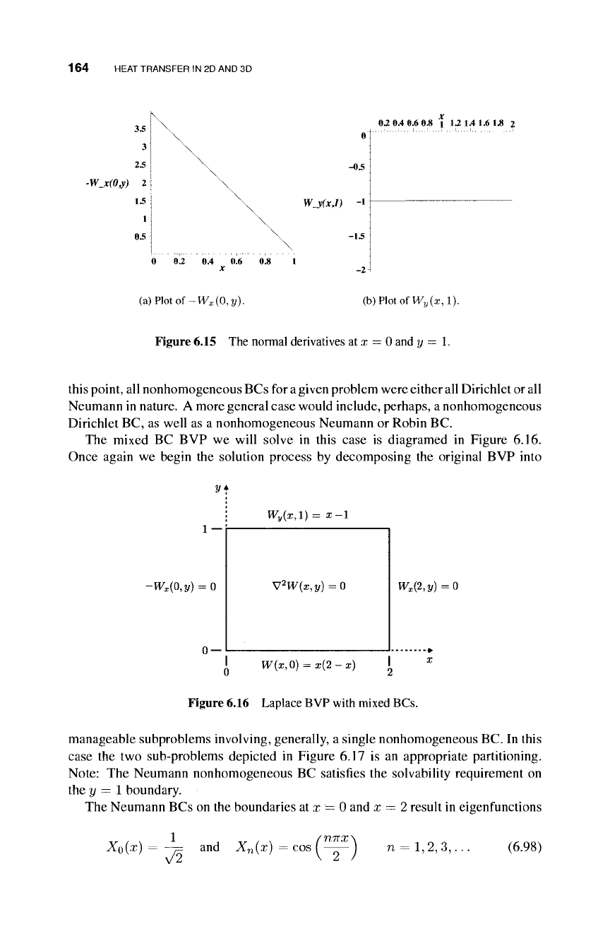
The normal derivative of W(x, y) at the other two boundaries is plotted in Figure

6.15.

This provides evidence that the solution for W(x,y) satisfies the required

boundary conditions for the faces.

6.4.5 Dirichlet, Neumann BC Example

This section provides an example of how we go about solving a 2D heat transfer

problem for which nonhomogeneous boundary conditions are mixed in type. Up to

164 HEAT TRANSFER IN 2D AND 3D

02 0.4 0.6 0.8 l 12 1.4 1.6 1.8 2

W_y(xJ)

-1

-15

(a)

Plot of-W*(0,0).

(b)PIotofW

(x,l).

Figure 6.15 The normal derivatives at x = 0 and y = 1.

this point, all nonhomogeneous BCs for

given problem were either all Dirichlet or all

Neumann in nature. A more general case would include, perhaps, a nonhomogeneous

Dirichlet BC, as well as a nonhomogeneous Neumann or Robin BC.

The mixed BC BVP we will solve in this case is diagramed in Figure 6.16.

Once again we begin the solution process by decomposing the original BVP into

-W

{0,y)

= 0

(x,l)=

x-1

W(x,y)

= 0

(2,y)=0

W(x,0) = x(2-x)

Figure 6.16 Laplace BVP with mixed BCs.

manageable subproblems involving, generally, a single nonhomogeneous BC. In this

case the two sub-problems depicted in Figure 6.17 is an appropriate partitioning.

Note: The Neumann nonhomogeneous BC satisfies the solvability requirement on

the y = 1 boundary.

The Neumann BCs on the boundaries at x

—

0 and x = 2 result in eigenfunctions

θ(

) = -/=

and

n(x) = COS (^2~)

n =

1,2,3,...

(6.98)

2D BVP: LAPLACE AND POISSON EQUATIONS 165

</*

-W

(0,y) = 0

(x,l)=

x-1

W(x,y)

= 0

(2,y)=0

W(x,0) = 0

(a) Subproblem one.

2/f

-W

(0,y) = 0

(x,l)=0

W{x,y)=0 W

(2,y)=0

W(x,0)=x(2-x)

(b) Subproblem two.

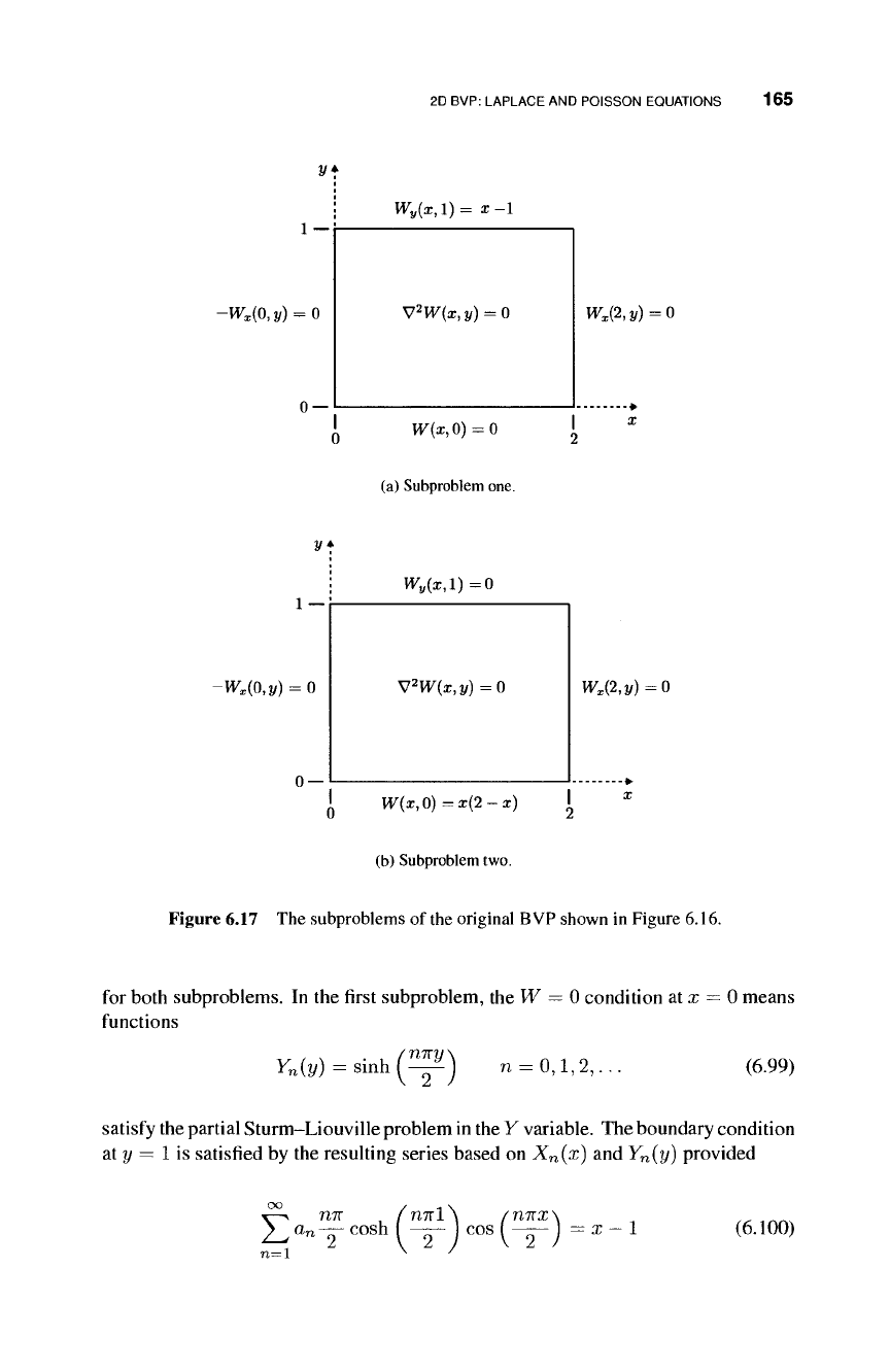
Figure 6.17 The subproblems of the original BVP shown in Figure 6.16.

for both subproblems. In the first subproblem, the W

—

0 condition at x = 0 means

functions

(y) = sinh (^p) n = 0,1,2,...

(6.99)

satisfy the partial Sturm-Liouville problem in the Y variable. The boundary condition

at y = 1 is satisfied by the resulting series based on X

(x) and Y

(y) provided

ηπ

/ηπΐλ

/ηπχ\

— cosh I — Icos [-γ-) =x-l

n=l ^ '

(6.100)

166 HEAT TRANSFER IN 2D AND 3D

which is the case if

2 f /

Τ17ΓΧ

rcosh(^)y

(*-1)οοβ(—)ώ (6.101)

Therefore, the solution VF

(x, y) for the first sub-problem is

W\x,υ)

Σα

cos

(ψ)

sinh

(ψ) , (6.102)

n=l

The Y

(y) functions that solve the partial Sturm-Liouville problem for the second

subproblem are

(y) = cosh

n7r(1

~^l

n = 0,1,2,... (6.103)

because of the homogeneous Neumann condition at y = 1. The solution for the

second subproblem is

,y)

= f>„ cos (^) cosh (^ί^) (6.104)

n=0

where the coefficient a

are

ou =

^í4f)í

i(2

i)cos

l05)

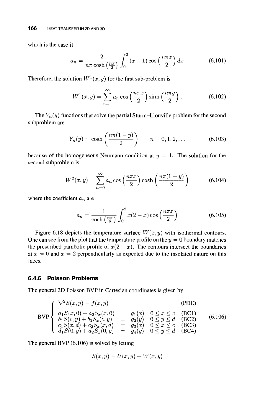
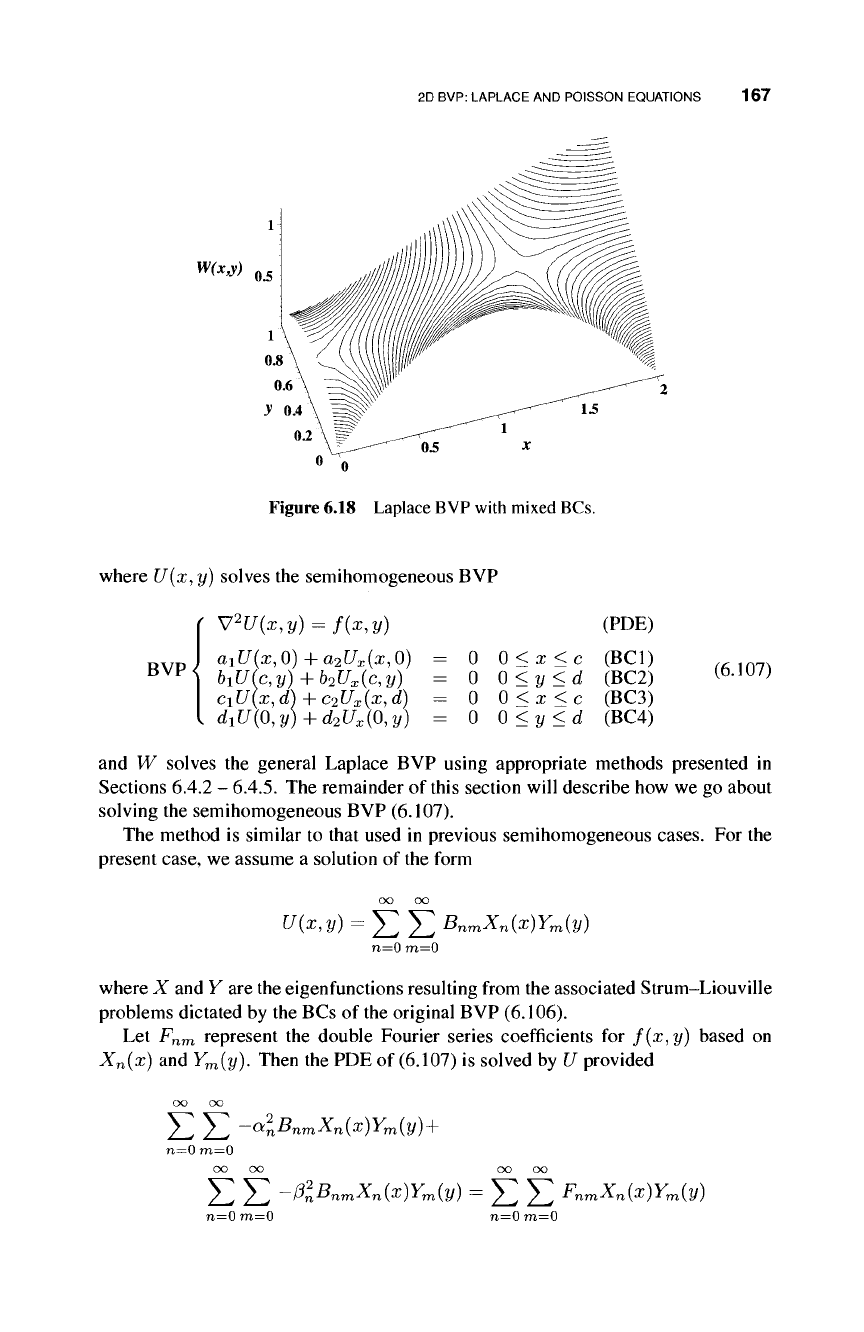
Figure 6.18 depicts the temperature surface W(x,y) with isothermal contours.

One can see from the plot that the temperature profile on the y

—

0 boundary matches

the prescribed parabolic profile of x(2

—

x). The contours intersect the boundaries

at x = 0 and x = 2 perpendicularly as expected due to the insolated nature on this

faces.

6.4.6 Poisson Problems

The general 2D Poisson BVP in Cartesian coordinates is given by

( \7

S(x,y) = f(x,y) (PDE)

S(x,0)+a

(x,0) =

(x) 0<x<c (BC1)

S(c,y)+b

(c,y) = M 0<y<d (BC2)

(

6J06

)

ci5(x, d) + c

(x,d) = g

(x) 0 < x < c (BC3)

1^5(0,^

+ ^^(0^) = g¿y) 0<y<d (BC4)

BVP^

The general BVP (6.106) is solved by letting

S{x,y) = U{x,y) + W{x,y)

2D BVP: LAPLACE AND POISSON EQUATIONS 167

W(xjr)

Figure 6.18 Laplace BVP with mixed BCs.

where U(x,y) solves the semihomogeneous BVP

BVP<

U(x,y)

= f(x,y)

aiU(x,0) +a

(x,0)

biU(c,y) + b

(c,y)

c\U{x, d) + C2Ü

(x, d

U(0,y)+d

(0,y

0 0 <x<c

0 0<y<d

0 0 <x<c

0 0 <y<d

(PDE)

(BC1)

(BC2)

(BC3)

(BC4)

(6.107)

and W solves the general Laplace BVP using appropriate methods presented in

Sections 6.4.2 - 6.4.5. The remainder of this section will describe how we go about

solving the semihomogeneous BVP (6.107).

The method is similar to that used in previous semihomogeneous cases. For the

present case, we assume a solution of the form

oo oo

U(x,y) = 2^2_^ B

nrn

(x)Y

(y)

n=0 m=0

where X and Y are the eigenfunctions resulting from the associated Strum-Liouville

problems dictated by the BCs of the original BVP (6.106).

Let

nrn

represent the double Fourier series coefficients for f(x,y) based on

(x)

and Y

(y). Then the PDE of (6.107) is solved by U provided

]T ]T -a

nrn

(x)Y

(y)+

oo oo oo oo

Σ Σ -ßlB

{x)Y

{y) = Σ Σ F

mXn{x)Ym{y)

n=0 m=0

oo oo

n=0 m=0 n=0 m=0

168 HEAT TRANSFER IN 2D AND 3D

which means

+ 0

n = 1,2,3,... andm = 1,2,3,...

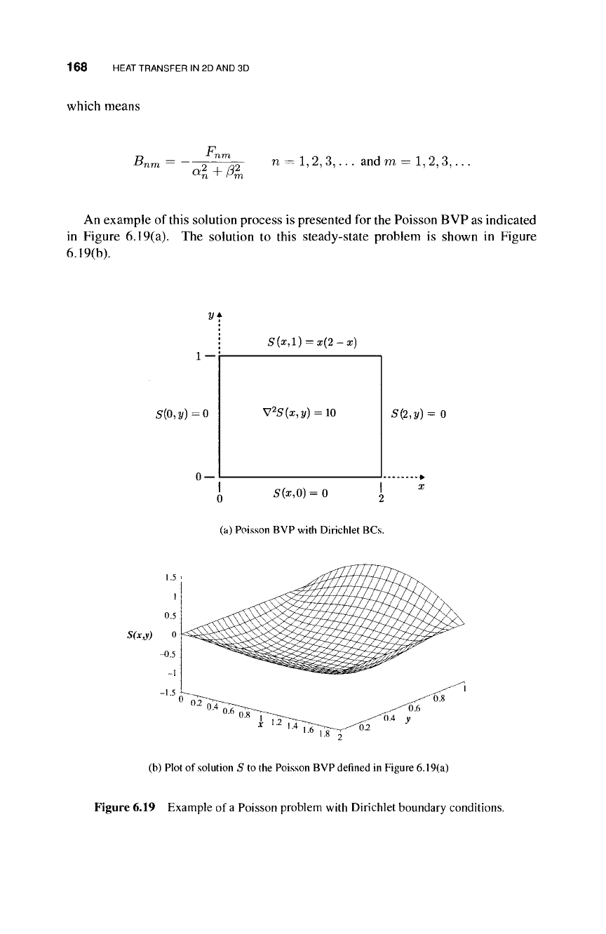
An example of this solution process is presented for the Poisson B VP as indicated

in Figure 6.19(a). The solution to this steady-state problem is shown in Figure

6.19(b).

2/f

5(0,2/) =0

S{x,l) =x{2-x)

S(x,y)

=10

S(2,y)= 0

5(x,0)=0

(a) Poisson BVP with Dirichlet BCs.

(b) Plot of solution S to the Poisson BVP defined in Figure 6.19(a)

Figure 6.19 Example of a Poisson problem with Dirichlet boundary conditions.

NONHOMOGENEOUS 2D EXAMPLE 169

6.5 NONHOMOGENEOUS 2D EXAMPLE

The details for solving the nonhomogeneous 2D IBVP 6.108 are provided in this

section.

ut = 0.1 [u

+ u

] (PDE)

u{x, y, 0) =

#[0.4,0.6] x [o.4,o.6]

(x, y) (IC)

(x, 0,t) = 0 0 < x < 1 (BC1) (6.108)

u(l,y,t) = 4y(l-y) 0<y<l (BC2)

î/

(x,l,i) = l/2-x 0<χ<1 (BC3)

I u(0, y, i) = 0 0 < y < 1 (BC4)

The solution u is assumed to be of

the

form u(x, y, t) — U(x, y, t) + W(x, y), where

W solves

IBVP<

(x,y)

= 0 (PDE)

BVP

Wy(X,0,t) = 0

W(l,y,t)=4y(l-

(x,l,t)

= l/2-

W(0,y,t)=0

-y)

- X

0 <x < 1

0 < 2/ < 1

0<£< 1

0<t/ < 1

(BC1)

(BC2)

(BC3)

(BC4)

(6.109)

the Laplace BVP 6.109 that includes the nonhomogeneous BCs given in IBVP 6.108,

and U solves the IBVP 6.110 with homogeneous forms of the nonhomogeneous BCs

of 6.108

IBVP<

=0.1[l/

+ ü

yi/

]

U(x,y,0) =

#[o.4,o.6] x [0.4,0.6]

(x,y) - W(x,y)

(x,0,t)

C/(l,j/,t) = 0

(x,l,t)=0

t/(0,y,i) = 0

(PDE)

(IC)

(6.110)

0 < x < 1 (BC1)

0 < y < 1 (BC2)

0 < x < 1 (BC3)

0 < y < 1 (BC4)

The solution for VF is determined by the methods outlined in Section 6.4.5.

Two subproblems, one each for the nonhomogeneous BCs, must be solved. The

eigenfunctions in this case are X

(x) — sin(a

x), with a

= ηπ (n =

1,2,3,...),

and Y

(y) = 1 for β

= 0, Y

(y) = cos(ß

y), for ß

= πιπ (m =

1,2,3,...).

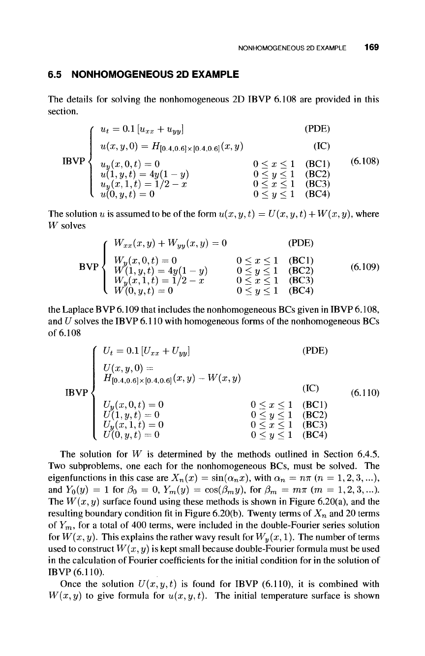
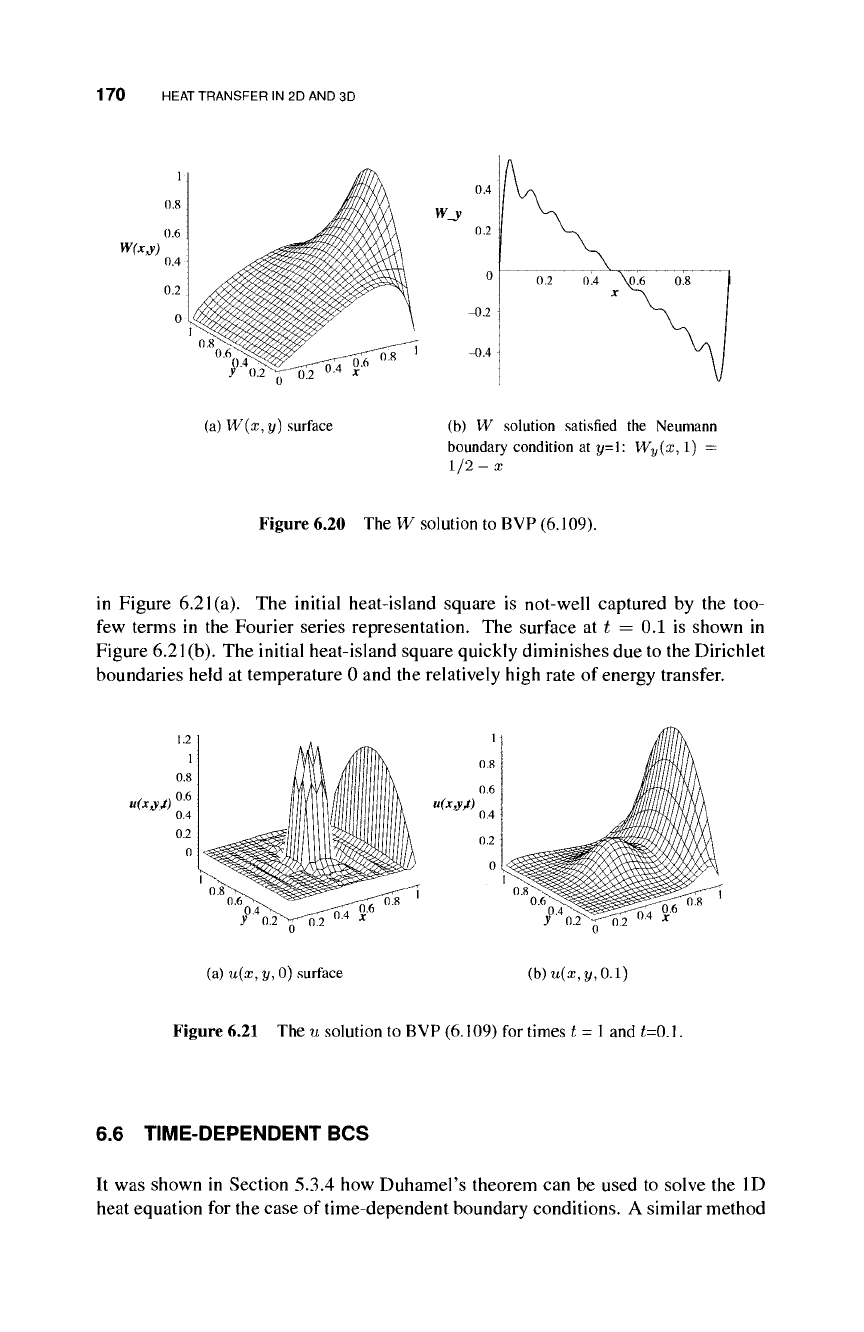
The W(x, y) surface found using these methods is shown in Figure 6.20(a), and the

resulting boundary condition fit in Figure 6.20(b). Twenty terms of X

and 20 terms

of Y

, for a total of 400 terms, were included in the double-Fourier series solution

for W(x, y). This explains the rather wavy result for W

(x, 1). The number of terms

used to construct W(x,y) is kept small because double-Fourier formula must be used

in the calculation of Fourier coefficients for the initial condition for in the solution of

IBVP (6.110).

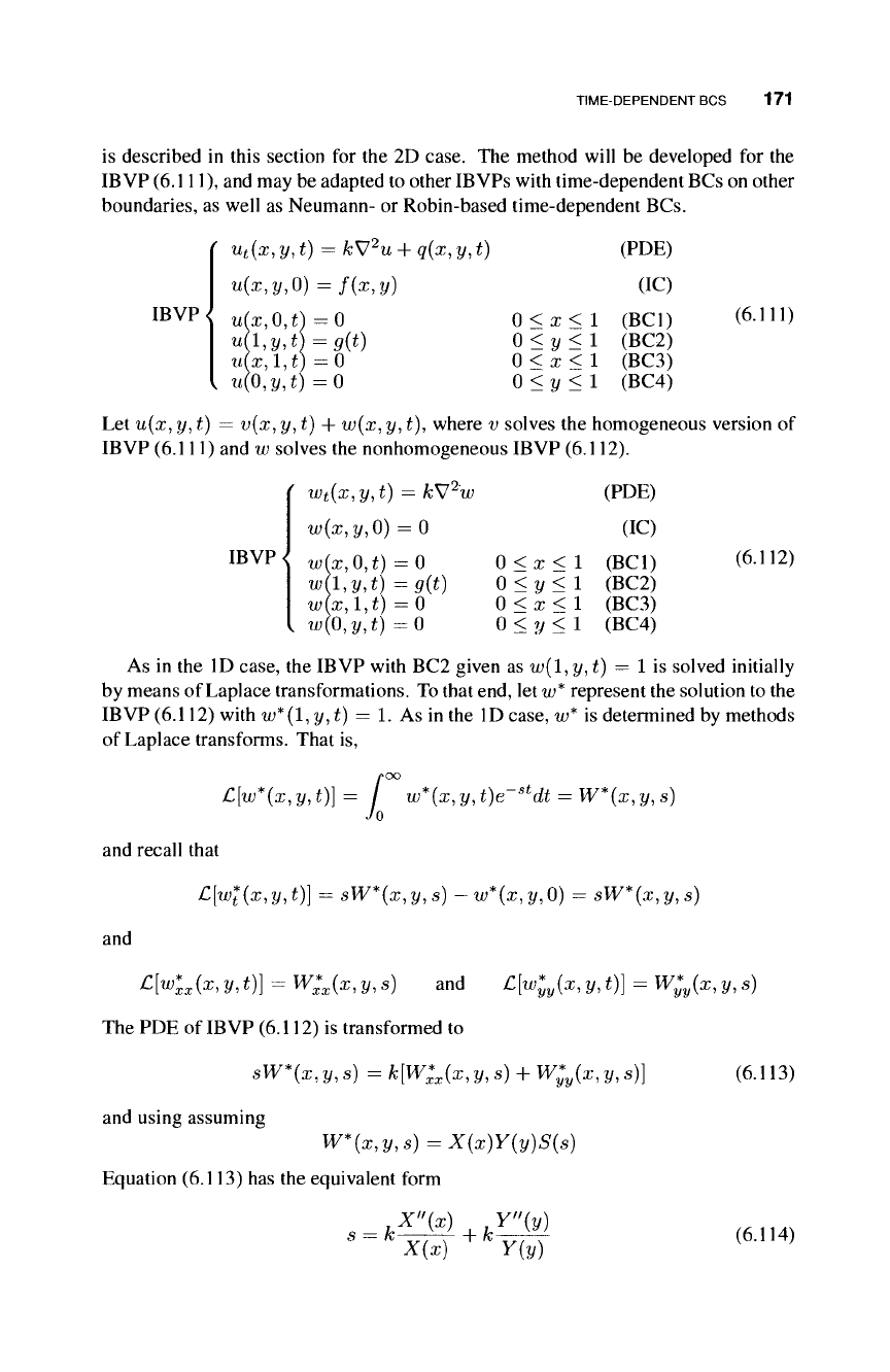
Once the solution U(x,y,t) is found for IBVP (6.110), it is combined with

W(x,y) to give formula for u{x,y,t). The initial temperature surface is shown

170 HEAT TRANSFER IN 2D AND 3D

W(x,y)

(b) W solution satisfied the Neumann

boundary condition at y=\: W

(x, 1) =

1/2-a;

Figure 6.20 The W solution to BVP (6.109).

in Figure 6.21(a). The initial heat-island square is not-well captured by the too-

few terms in the Fourier series representation. The surface at t = 0.1 is shown in

Figure 6.21(b). The initial heat-island square quickly diminishes due to the Dirichlet

boundaries held at temperature 0 and the relatively high rate of energy transfer.

u(xyjt) u(x,yjt)

y 0.2>j^0.2

(á)u(x,y, 0) surface (b)u(x,y,0.1)

Figure 6.21 The u solution to BVP (6.109) for times t = 1 and

£=0.1.

6.6 TIME-DEPENDENT BCS

It was shown in Section 5.3.4 how Duhamel's theorem can be used to solve the ID

heat equation for the case of time-dependent boundary conditions. A similar method

TIME-DEPENDENT BCS 171

is described in this section for the 2D case. The method will be developed for the

IBVP

(6.

Ill), and may be adapted to other IBVPs with time-dependent BCs on other

boundaries, as well as Neumann- or Robin-based time-dependent BCs.

IBVP<

( u

(x,y,t) = kV

u-\-q(x,y,t)

u{x,y,0) = f(x,y)

u(x,0,t)

—

uh,y,t) = g(t)

u(x, l,i) =0

I tfc(0,2/,i) =0

(PDE)

(IC)

0 < x < 1 (BC1)

0 < y < 1 (BC2)

0 < x < 1 (BC3)

0 < y < 1 (BC4)

(6.111)

Let u{x, y, t) — v(x, y, t) + w(x, y, f), where v solves the homogeneous version of

IBVP (6.111) and w solves the nonhomogeneous IBVP (6.112).

IBVP<

( w

(x,y,t) — kV

w(x,y,0) =0

w(x,0,t) = 0

wh,y,t) =g(t)

w(x, l,f) = 0

I w{0,y,t) = 0

(PDE)

(IC)

0<x<l (BC1)

0 < y < 1 (BC2)

0 < x < 1 (BC3)

0 < y < 1 (BC4)

(6.112)

As in the ID case, the IBVP with BC2 given as w(l, y, t) — 1 is solved initially

by means of Laplace transformations. To that end, let

represent the solution to the

IBVP (6.112) with w*(l,y,t) — 1. As in the ID case, w* is determined by methods

of Laplace transforms. That is,

/»OO

C[w*{x,y,t)]= / w*(x,y,t)e-

dt =

W*(x,y,s)

and recall that

C[wl(x,y,t)\

= sW*(x,y,s) -w*(x,y,0) = sW*(x,y,s)

and

¿Κ^ι/,ί)]

xx(

,yi

)

and

£[u>lyfay,t)] =

(x,

,s)

The PDE of IBVP (6.112) is transformed to

sW*(x,y,s) = k[W;

(x,y,s) +

(x,y,s)]

(6.113)

and using assuming

W*(x,y,s)

= X(x)Y(y)S(s)

Equation (6.113) has the equivalent form

X(x) Y(y)