Bernatz R. Fourier Series and Numerical Methods for Partial Differential Equations

Подождите немного. Документ загружается.

152 HEAT TRANSFER IN 2D AND 3D

Substituting for W

given by Equation (6.42) into Laplace's equation, and dividing

both sides of the resulting equation by X(x)Y(y) gives

X(a:)

y(y)

X(x) Y(y) ^

We introduce the separation constant —λ, and Equation (6.43) is split into the fol-

lowing second-order ODEs

X"(x)

+ XX(x)

= 0

(6.44)

Y"(y)-XY(y)

= 0

(6.45)

The zero Dirichlet BCs result in eigenvalues of λ

— (—) (n

1,2,3,...)

and eigenfunctions X

(x) = sin a

x. Now that values for λ are known, the ODE in

Y becomes

Y"(y)

Y(y) = 0 (6.46)

which has the general solution

Y(y)

Be-°

(6.47)

Invoking the BC at y

—

0, we have

y (0)

"°

Be"*"

=0^A

+ ß =

0=^5

-A (6.48)

so that the solution for

reduces to

Y(y)

2A sinh a

y (6.49)

or, more simply

Y(y) = A sinh a

y (6.50)

complete the solution process for subproblem

the

boundary condition W

(x,

g%{x)

must be satisfied. That is, we require

/2~

(x,d)

W-sin(a

x)sinh(a:

d) = gz{x) (6.51)

sinh(a

sin(a

(x) (6.52)

which is possible by letting

-Γ-Γ,

-77 A

-sin(a

x)dx (6.53)

smh(a

Note \7

(x, y)

0 on the rectangular domain

[0,

d].

(x, d) = #3,

and VF

(x, y) is identically zero on the other three boundaries.

2D BVP: LAPLACE AND POISSON EQUATIONS 153

Next, we search for a solution W

(x,y). Assuming

{x,y)

= X(x)Y(y) as

in the previous subproblem, we know X

(x) — sm(a

x) with a

= ™ (n =

1,2,3,...).

In terms of Y

{y), the general solution remains

(y) = Ae

anV

+ Be-

(6.54)

but Y

{y) must be zero at y = d instead of y = 0 as before. This suggests the

possibility of letting

(y) = Ae

an{d

+ Be~

(6.55)

If so, then it remains that Y"{y)

—

Y(y) = 0. Invoking the zero boundary

condition at y = d gives

(d) = Ae

4- Be-

an{d

= 0

B = -A (6.56)

so that

(y) = Asmh(d-y) (6.57)

The formula

(x, y) = ^2

sm{a

x) sinh(a

(d - y)) (6.58)

n=l

solves all but the nonhomogeneous BC of subproblem 1. This boundary condition is

satisfied by requiring

(x,0)

^2b

J-

sm(a

x) sinh(a

(d) = gi(x) (6.59)

71=1

which is true for

n= -Τ-Γ7—^\-sm(a

x)dx (6.60)

sinh(a

This is the same requirement we found for b

in subproblem 3, except there g^{x)

took the place oïg\{x) as indicated in Equation (6.53).

reasonable to expect similar solutions exist for W

and W

. Without providing

extensive details, these solutions are

OO ΠΖ

(x,y)

Y2b

J-

sm(a

y) sinh(a

x) (6.61)

i ·

n=l

with

and

\JlM<*

y)dy

(6.62)

sinn(a

°° 12

(x,y)

= ^b

J- sm(a

y) sinh(a

(c - x)) (6.63)

n=l

154 HEAT TRANSFER IN 2D AND 3D

with

sinh(a

sin(a

y)dy

(6.64)

An example of these procedures will be presented next. However, it is an ap-

propriate time to make a couple of comments about the solution W of the original

BVP shown in Figure 6.5. The first is that the solution for W in a Dirichlet problem,

such as this, is unique. This statement is made without

proof.

However, it can be

understood to be true in the same way we know that the second-order BVP of the

ODE

y"(x)

= 0 (a < x < b) and y (a) = y

y(b) = y

has a unique solution.

The second comment concerns the role W(x, y) plays in certain IBVPs. Suppose

we are given a general IB VP with Dirichlet BCs, none of which are time dependent.

Following the methods described so far, we determine u{x,y,t) = U(x,y,t) +

W(x,y)

where U solves a semihomogeneous IBVP, and W solves the Dirichlet

BVP based on Laplace's equation. The time-dependant term U(x, y, t) will, in fact,

have limit zero as t tends to infinity. Therefore, the function W(x, y) represents the

limiting, steady-state temperature solution of the rectangular domain.

6.4.2 Dirichlet Example

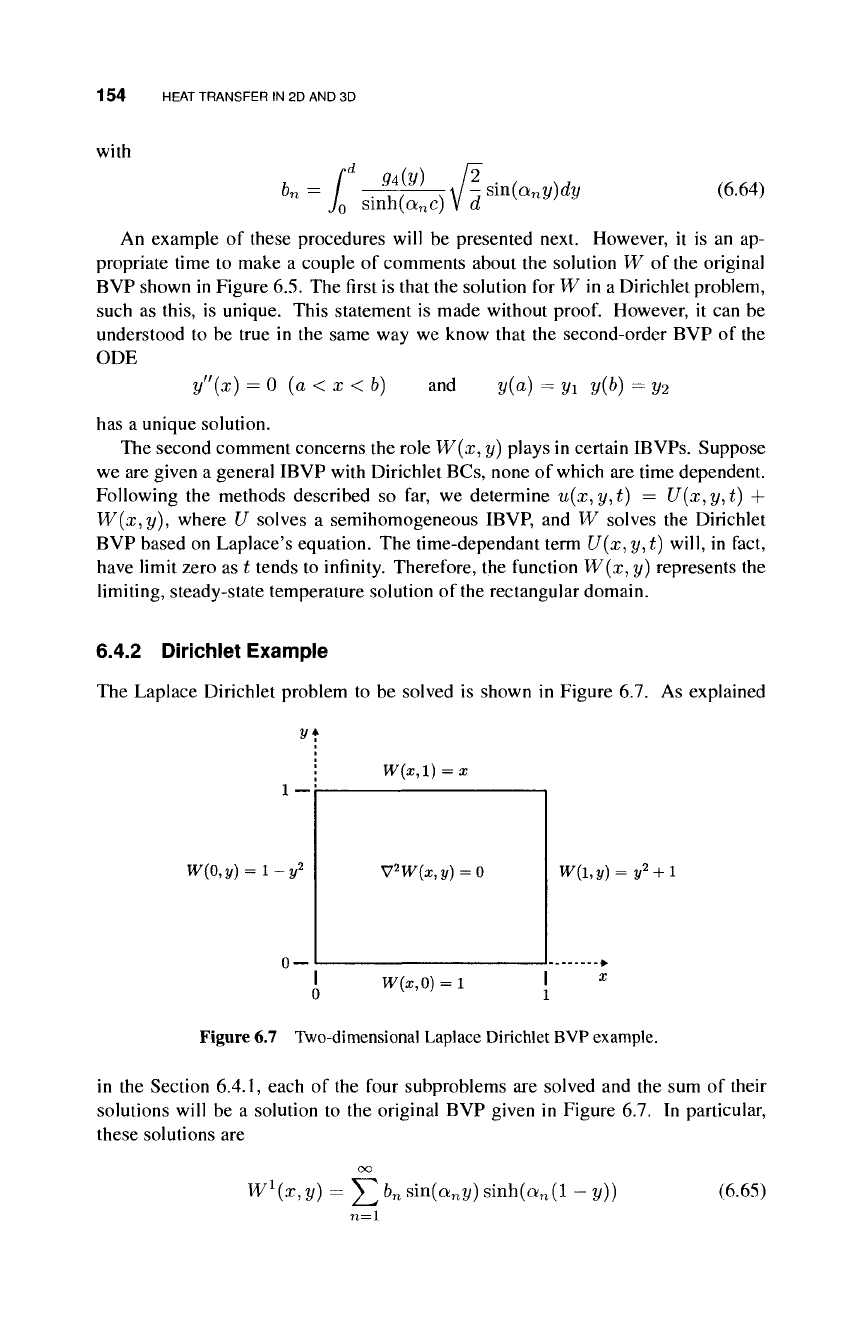
The Laplace Dirichlet problem to be solved is shown in Figure 6.7. As explained

W{x,l) = x

^(0,2/) = 1

W{\,y) = y

+ l

Figure 6.7 Two-dimensional Laplace Dirichlet BVP example.

in the Section

6.4.1,

each of the four subproblems are solved and the sum of their

solutions will be a solution to the original BVP given in Figure 6.7. In particular,

these solutions are

(x,y)

= Y^b

sin(a

y)smh(a

(l - y))

(6.65)

n=l

2D BVP: LAPLACE AND POISSON EQUATIONS 155

with

ηπ

and b

= -—-.—— sm(a

x)dx

sinh(a

(x,y)

= ^ b

V2sin(a

y) sinh(a

(x)) (6.66)

n=l

with

= ηπ

;

and b

— \ —— r sin(a

y)dy

sinh(a

V ny) y

(x, y) = Y^b

sin(a

x) sinh(a

(l - y))

(6.67)

n=l

with

and

with

Οί

f x

and b

= —— sin(a

x)dx

sinh(a

(x,y)

= ^ b

V2sm(a

y) sinh(a

(2 - x))

n=l

1-y

and b

= -—-—— sin(a

y)dy

smh(a

(6.68)

= ηπ

;

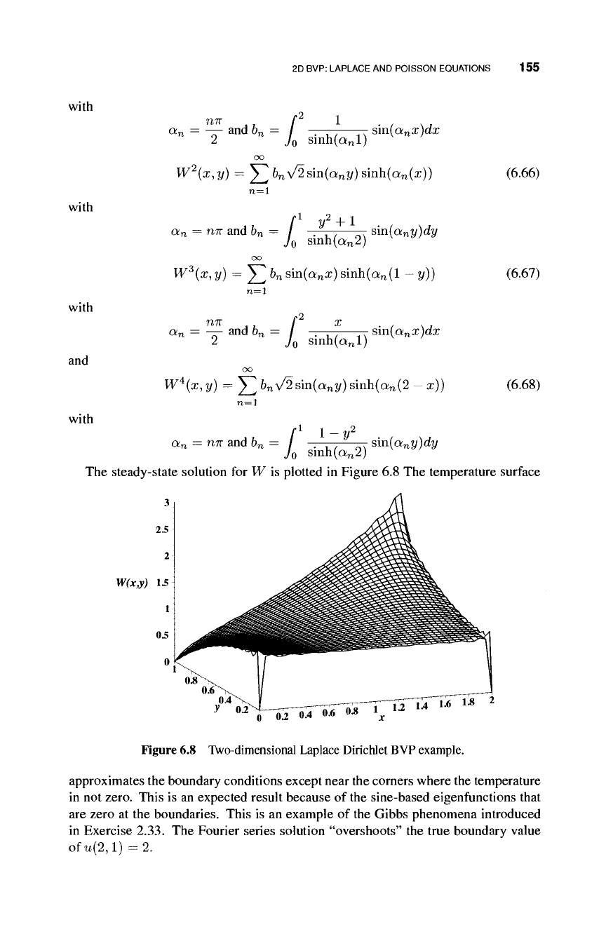
The steady-state solution for W is plotted in Figure 6.8 The temperature surface

3Ί

Figure 6.8 Two-dimensional Laplace Dirichlet BVP example.

approximates the boundary conditions except near the corners where the temperature

in not zero. This is an expected result because of the sine-based eigenfunctions that

are zero at the boundaries. This is an example of the Gibbs phenomena introduced

in Exercise 2.33. The Fourier series solution "overshoots" the true boundary value

of i/(2,l) = 2.

156 HEAT TRANSFER IN 2D AND 3D

6.4.3 Neumann Problems

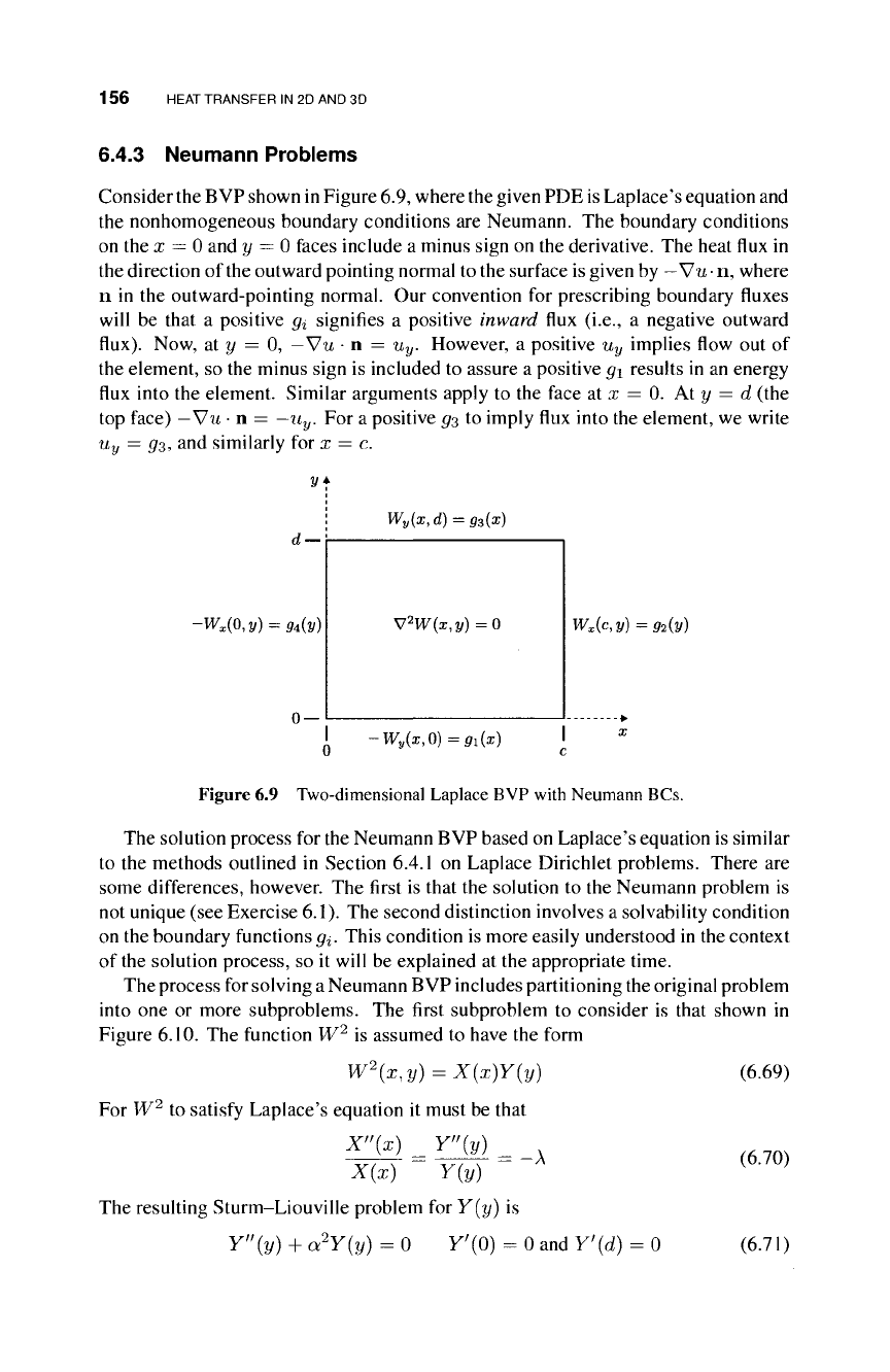
Consider the BVP shown in Figure 6.9, where the given PDE is Laplace's equation and

the nonhomogeneous boundary conditions are Neumann. The boundary conditions

on the x

—

0 and y = 0 faces include a minus sign on the derivative. The heat flux in

the direction of the outward pointing normal to the surface is given by — Vu

n, where

n in the outward-pointing normal. Our convention for prescribing boundary fluxes

will be that a positive gi signifies a positive inward flux (i.e., a negative outward

flux). Now, at y = 0, — Vu · n = u

. However, a positive u

implies flow out of

the element, so the minus sign is included to assure a positive

results in an energy

flux into the element. Similar arguments apply to the face at x = 0. At y = d (the

top face) —Vu · n = — u

. For a positive gs to imply flux into the element, we write

Uy =93, and similarly for x

—

(x,d)

=93(x)

-W

(0,y) = g

(y)

W(x,y)

= 0

-W

(x,0)=

(x)

(c,y)

(y)

Figure 6.9 Two-dimensional Laplace BVP with Neumann BCs.

The solution process for the Neumann BVP based on Laplace's equation is similar

to the methods outlined in Section 6.4.1 on Laplace Dirichlet problems. There are

some differences, however. The first is that the solution to the Neumann problem is

not unique (see Exercise

6.1

The second distinction involves a solvability condition

on the boundary functions

#¿.

This condition is more easily understood in the context

of the solution process, so it will be explained at the appropriate time.

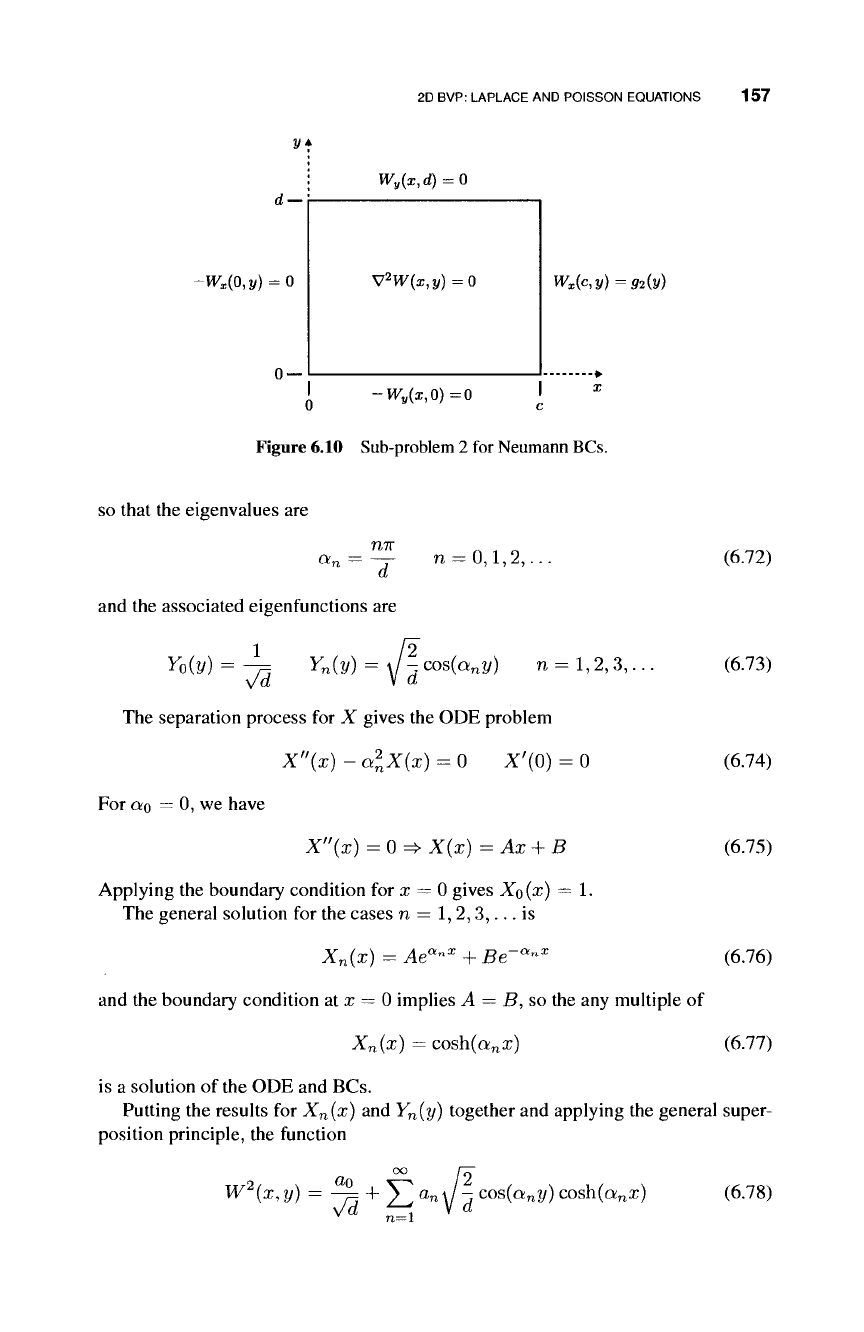
The process for solving

Neumann BVP includes partitioning the original problem

into one or more subproblems. The first subproblem to consider is that shown in

Figure 6.10. The function W

is assumed to have the form

(x,y)

= X(x)Y(y)

-X

For W

to satisfy Laplace's equation it must be that

X"{x)

Y"{y)

X(x) Y(y)

The resulting Sturm-Liouville problem for Y(y) is

Y"(y) + a

Y(y) = 0 y'(0) = 0 and Y'(d) = 0

(6.69)

(6.70)

(6.71)

2D BVP: LAPLACE AND POISSON EQUATIONS 157

-W

(0,y) =

{x,d)

= 0

W(x,y)=0

-W

{x,0)=0

(c,y)

(y)

Figure 6.10 Sub-problem 2 for Neumann BCs.

so that the eigenvalues are

a„

ηπ

n = 0,l,2,...

and the associated eigenfunctions are

Yo(y)

1 2

— Y

(y) = d-cos(a

y) n = 1,2,3,...

The separation process for X gives the ODE problem

X"(x)

- a

X{x) = 0 X'(0) = 0

For ao = 0, we have

X"{x)

= 0 =» X(x) = Ax + B

Applying the boundary condition for x = 0 gives Xo{x) — 1.

The general solution for the cases n = 1,2,3,. ..is

(6.72)

(6.73)

(6.74)

(6.75)

(6.76)

(x)

= Ae

anX

4- Be-""*

and the boundary condition at x = 0 implies A = J3, so the any multiple of

^n0*0 = cosh(a

x) (6.77)

is a solution of the ODE and BCs.

Putting the results for X

(x) and Y

(y) together and applying the general super-

position principle, the function

{x,y)

= -J= ~{-

^2a

J-cos(a

y)cosh(a

n=l

(6.78)

158 HEAT TRANSFER IN 2D AND 3D

satisfies Laplace's equation and the three homogeneous BCs of subproblem 2.

Now we consider how the nonhomogeneous BC may be satisfied by W

(x, y).

(c,y)

= g

(y) => X^

W-

cos

(

nI/) sinh(a

c) = g

(y) (6.79)

n=i

Equation (6.79) is satisfied if the cosine series with coefficients a

sinh(a

matches the function #2(2/)· This is true provided

sinh(a

c) = / g

(y)J-cos(a

y)dy

1 f

Í2

=^^n = 7-r-, r /

(y)\

-cos(a

y)dy

smh{a

c) J

\ d

for n = 1,2,3,... and

(y)

■— dy = 0 (6.80)

d !

/o Vd

The integral in Equation (6.80) is the inner product of Yo(y) and g

(y) used to

determine the zero-order term in the cosine series representation of

(y).

The BC

requirement of Equation (6.79) has a vanishing zero-order term that is the case,

provided Equation (6.80) is satisfied. Consequently, the subproblem is solved using

this method provided

/ 92(y)dy = 0.

This is the "solvability" condition mentioned above. A similar requirement on gi

holds for the other three subproblems. The solvability condition is specific to the

given subproblem. The solvability condition for the original Neumann problem

shown in Figure 6.9 is

pc pd pc pd

/ #i(x)öb+ / g

(y)dy-\- / g

(x)dx + / g

(y)dy = 0 (6.81)

Jo Jo Jo Jo

The solution to subproblem 2 is complete with the satisfaction of the non-

homogeneous BC. The formal solution for W

(x, y) is

°° Í2

(x,y)

= a

4- y^ a

\ -cos(a

y) cosh(a

x) (6.82)

^-i Va

n=l

with

1 f

Í2

an = :

~T7 \ 92(y)\-,cos(a

y)dy n =

l,2,3,...

(6.83)

sinh(a

c) J

The constant ao is undetermined in this formulation because of

the

lack of uniqueness

of solution due to the boundary condition.

BVP: LAPLACE AND POISSON EQUATIONS 159

Each of the remaining subproblems are solved in a similar way. The formulas for

the solutions are given below. It will be left to the reader to fill in the details of each

solution process.

(x,y)

= qp+y^ a

\ - cos(a

x) cosh(a

(d-y)) a

= — n = 0,1,2,..

n=i

c c

(6.84)

with

™

^~τΤί—1\

9i(x)\

-cos(a

x)á

smh(a

d) J

V c

x n = 1,2,3,... (6.85)

, , , , ηπ

(x,y) = a

4- ^ a

y - cos(a

x) cosh(a

?/) a

= — n = 0,1,2,...

(6.86)

•

c c

n—l

with

n = 1,2,3,... (6.87)

™

^τ~ί—Λ\

/ 9Á

)\ -cos(a

x)dx

smh(a

d) J

V c

/IT

(x,y)

= a

+y^ a

\ - cos(a

y) cosh(a

(c-x)) a

= — n = 0,1,2,..

(6.88)

with

™

= r

~T^ \ / 94(y)\ -^cos(a

y)dy

sinh(a

c) J

V d

n = 1,2,3,... (6.89)

Now that each of

the

sub-problems have been solved, the full solution for W(x, y)

may be given as

W(x,y) = W

(x, y) + W

(x, y) +

(x,y)

+ W

(x,

j/)

(6.90)

6.4.4 Neumann Example

Consider the Neumann problem specified in Figure 6.11. The boundary conditions

indicate the rectangular material has insulated boundaries along y = 0 and x = 2.

There is a positive flux of energy along the face at x

—

0 and a negative flux at y

—

First, note the proposed problem satisfies the boundary solvability requirement in

that

/»2

/»l /*2 /»l

0-dx+ 0-dy+

-ldx+ 4(1 - y)dy = 0 + 0 + 2 - 2 = 0 (6.91)

JO JO JO

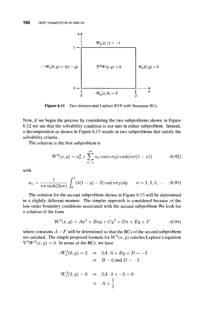
160 HEAT TRANSFER IN 2D AND 3D

-W,(0,y) = 4(l-y)

(x,l)=-1

W{x,y)

= 0

-Wy(x,0)

= 0

(2,y)

= 0

Figure

6.11

Two-dimensional Laplace BVP with Neumann BCs.

Now, if we begin the process by considering the two subproblems shown in Figure

6.12 we see that the solvability condition is not met in either subproblem. Instead,

a decomposition as shown in Figure 6.13 results in two subproblems that satisfy the

solvability criteria.

The solution to the first subproblem is

W (x, y) = a

+ y.

n cos(n7n/) cosh(n7r(l

—

x))

n=l

with

ηπ sinh(2n7r)

/ (4(1 - y) - 2) cos(nny)dy

n = 1,2,3,.

(6.92)

(6.93)

The solution for the second subproblem shown in Figure 6.13 will be determined

in a slightly different manner. The simpler approach is considered because of the

low-order boundary conditions associated with the second subproblem We look for

a solution of the form

(x, y) = Ax

+ Bxy + Cy

4- Dx + Ey

H-

F (6.94)

where constants A - F will be determined so that the BCs of

the

second subproblem

are satisfied. The simple proposed formula for W

(x, y) satisfies Laplace's equation

(x, y) = 0. In terms of the BCs, we have

-W

(0,y) = 2

0 + By + D = -2

B = 0 and D = -2

W*(2,y)

= 0

2,4-2-f-2 = 0

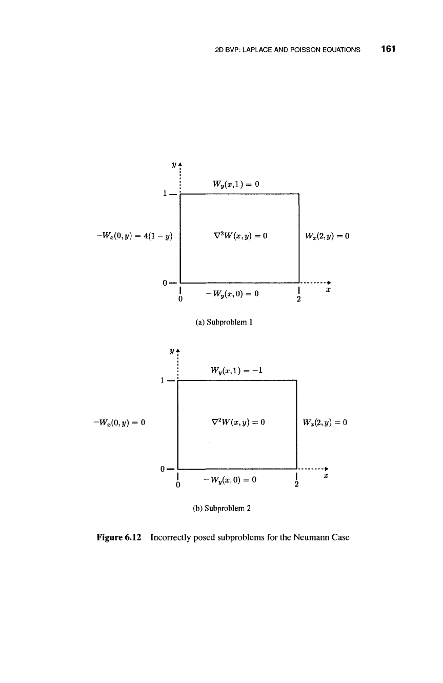
2D BVP: LAPLACE AND POISSON EQUATIONS 161

2/f

-W

(0,y) = 4(l-y)

(x,l)

= 0

W(x,y)

= 0

-W

(x,0) = 0

(a) Subproblem 1

(%y)

= 0

(x,l)

= -1

-W

(0,y) = 0

W{x,y)

= 0

-W

(x,0) = 0

(b) Subproblem 2

%y)=0

Figure 6.12 Incorrectly posed subproblems for the Neumann Case