Bernatz R. Fourier Series and Numerical Methods for Partial Differential Equations

Подождите немного. Документ загружается.

192

WAVE EQUATION

The solution formulation will be complete once expressions for A

(0) and B

(0)

are determined. We know the general solution for y(x, t) is given by Equation (7.40).

Matching the initial displacement f\ (x) when t = 0 gives

]T (A

(0) cos(ca

0) + B

(0) sin(ca

0)) X

(x) = f

(x)

^^^„(0)X

(x) = h{x)

n=0

(0) = Í

(x)X

(x)dx

Next, the initial velocity f%(x) is matched for t

—

0 to give

^2(A

(0)cos{ca

0) + B

(0)sm(ca

0)yX

{x) = f

(x)

n=0

J2ca

(0)X

(x) = f

(x)

n=0

(0) = —[

(x)X

(x)dx

Formulas for A

(t) and B

(t) given in (7.48) and (7.49) are valid for all n > 1.

The case for zero as an eigenvalue (λ = 0) must be treated separately because the

general solution to the ODE given by Equation (7.45) is given by linear combinations

of the solutions C\ — 1 and C

= t. In the event of a zero eigenvalue, the formulas

for Ao(t) and B

(t) are

(t)

= A)(0) + / -rFo(r) dr (7.50)

(t)=B

(0)+ Í F

(r)dr (7.51)

with

pL pL

A)(0)=/

{x)X

(x)dx

ana B

(0) =

(x)X

(x)dx

(7.52)

Jo Jo

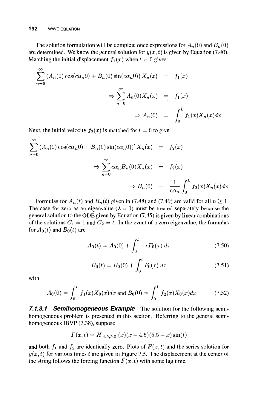
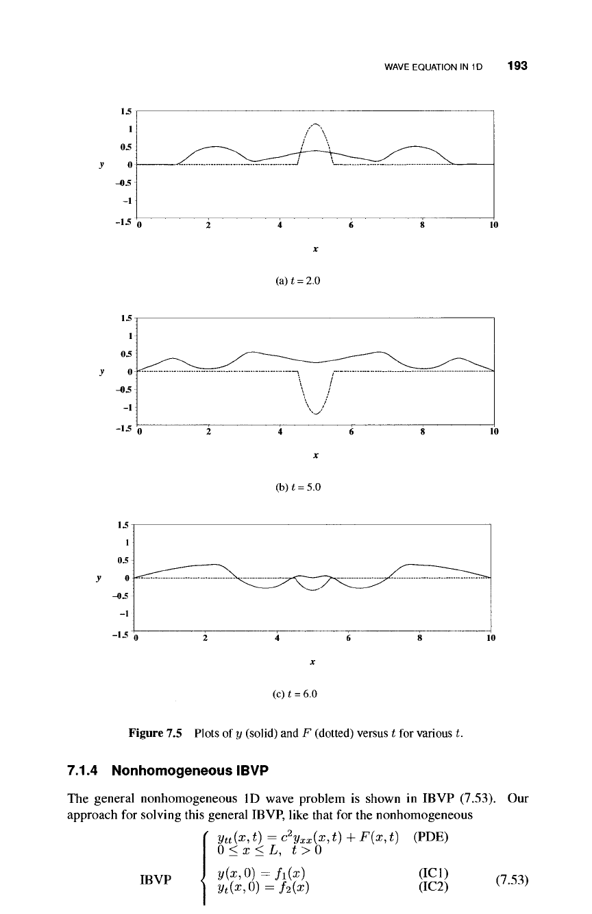
7.1.3.1

Semihomogeneous Example The solution for the following semi-

homogeneous problem is presented in this section. Referring to the general semi-

homogeneous IBVP (7.38), suppose

F(x, t) = if

[4.5,5.5]

0*0

(x - 4.5)(5.5 - x) sin(i)

and both f\ and f

are identically zero. Plots of F(x,t) and the series solution for

y(x,t) for various times t are given in Figure 7.5. The displacement at the center of

the string follows the forcing function F(x, t) with some lag time.

WAVE EQUATION IN 1D 193

(a)

2.0

(b)

5.0

(c)

6.0

Figure 7.5 Plots of y (solid) and F (dotted) versus t for various t.

7.1.4 Nonhomogeneous IBVP

The general nonhomogeneous ID wave problem is shown in IBVP (7.53). Our

approach for solving this general IBVP, like that for the nonhomogeneous

(x,t)

{x,t)

+ F(x,t) (PDE)

0 < x < L, t>0

IBVP

y(x,0) = f

(x)

yt(x,0) = /

(x)

(ICI)

(IC2)

(7.53)

194

WAVE EQUATION

ID heat equation, is to assume a solution of the form

y(x, t) = y

(x,

t) + S(x, ¿) (7.54)

where S(x,t) satisfies the nonhomogeneous BCs of the IBVP. If so, the function

Y(x,t) is left to solve a semihomogeneous wave problem. Such a solution may be

determined using methods of Section 7.1.3.

A suitable form of 5(x, t) in many instances is

S(x,t) = A(t) + B(t)x (7.55)

where A(t) and B(t) are determined by satisfying BC1 and BC2. Assuming this

may accomplished, we identify the resulting semihomogeneous problem that Y(x,t)

must solve.

Substituting for y and its derivatives in the PDE of IBVP (7.53), we have

Ytt{x, t) + A"{t) + B"{t)x = c

(x, t) + F(x, y) (7.56)

which leads to the PDE

Ytt(x,t) = c

(x,t) + F*(x,y) (7.57)

where

F*(x, y) = F(x, y) - A"{t) - B"{t)x (7.58)

Next, we substitute the proposed form for y(x,t) in the initial conditions prescribed

in IBVP (7.53) to determine the initial conditions required of Y(x,t). For initial

condition

(IC1 ),

we have

y(x,0) + A(0) + B(0)x = h(x) => y(x,0) = f¡(x) (7.59)

where

/í(x) - h(x) - ^(0) - B(0)x (7.60)

For initial condition (IC2), we have

(x,0) 4- ^(0) + B'(0)x = f

(x)

Yt(x,0) = r

{x) (7.61)

where

*(*) =

Λ(Χ)

- ^'(0) - B'(0)x (7.62)

A simple nonhomogeneous example is solved in Section

7.1.4.1.

7.1.4.1 Nonhomogeneous Example The simple nonhomogeneous problem

prescribed in IBVP (7.63) is solved in this section. The stretched string in this

example

(

(x,t)

= 2y

(x,t) (PDE)

| 0 < x < 10, t > 0

!/(x,0)=0 (ICI)

î/t(x,0)=0 (IC2)

)

y(0,t) = ^siní (BCl)

I 2/(10,*) =0 (BC2)

IBVP<

WAVE EQUATION IN 1D 195

has no initial displacement nor initial velocity. Note the PDE of IBVP (7.63) is ho-

mogeneous as well as boundary condition (BC2). The latter translates to a stationary

right end point for the string. However, boundary condition (BCl) implies the left

end of the string oscillates on the ?/-axis between

— ^

and |.

Requiring S(x, t) = A(t) 4- B(t)x to satisfy both boundary conditions gives

A(t) = -sini and B(t) = -——— sint

Once A(t) and B(t) have been determined, formulas for F*(x, t), fl(x), and /! (#)

can be found. In this case,

F*(x,t) = -sint

—

x sini

)

2 2-10

fi(x) = -isinO + x—^sin0 = 0

1 1 1 x

fo(x) = --cosO -\-x——— cosO =

—

- 4- —

J2K )

2 2-10 2 20

The homogeneous Dirichlet BCs of the resulting semihomogeneous IBVP for

Y(x,t) require eigenfunctions and eigenvalues

2 77/7Γ

— sin(a

x) a

= —, n = 1,2,3, ...

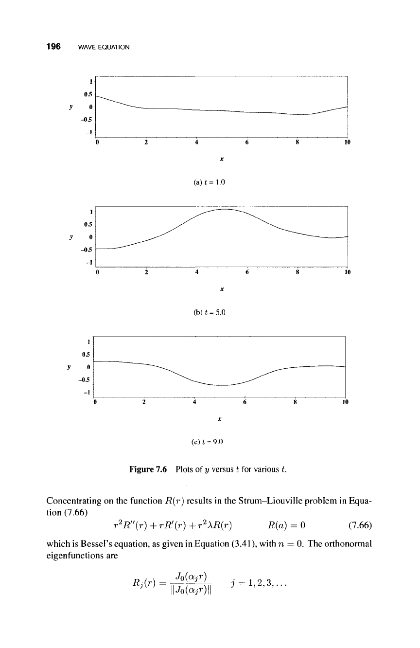
Figure 7.6 shows the string's displacement for various times t. The left end of the

string at x

0 oscillates, as prescribed, between the values of

—

\ and \ as the right

end point remains stationary.

7.1.5 Homogeneous IBVP in Polar Coordinates

The solution process for homogeneous ID initial boundary value problem in polar

coordinates is presented in this section. The specifics of the problem are shown in

IBVP (7.64).

ztt(r, t) = c

(r, t) + \z

(r, t)) (PDE)

0 < r < a, t > 0

IBVP<

*(r,0) = /i(r) (ICI)

(J M)

*t(r,0) = /

(r) (IC2)

ö4)

z(a,t)=0 (BCl)

|y(r,f)|<oo (BC2)

The initial displacement is given by /i(r) and the initial velocity by f

{r) of the

surface. The boundary condition at r = a is homogeneous and Dirichlet.

A separated solution of the form z(r, t) = R(r)T(t) is sought. Subbing for z in

the PDE, simplifying, and introducing the separation constant λ gives

Ht) fi^fr) l^(r)

T{t) R(r)

r R(r)

(

196

WAVE EQUATION

(a)t=1.0

(b) t = 5.0

Figure 7.6 Plots of y versus t for various t.

Concentrating on the function R(r) results in the Strum-Liouville problem in Equa-

tion (7.66)

R"{r)

+ rR'(r) +

XR(r)

R(a) = 0 (7.66)

which is Bessel's equation, as given in Equation (3.41), with n = 0. The orthonormal

eigenfunctions are

Rj(r)

Jo(ajr)

3 =

1,2,3,...

WAVE EQUATION IN 1D 197

where the eigenvalues aj are the zeros of the Bessel function Jo(ar).

Now that the eigenvalues are known from the R equation, the differential equation

for T found from Equation (7.65) is

T"(t) + c

a]T{t) = 0 (7.67)

with general solution

T(t) = Aj cos(cajt) + Bj sin(ca¿í) (7.68)

Combining the results for R and T gives the Fourier solution for z(r,t) shown in

Equation (7.69).

(

i ¿) = Σ(

cos

(

) +

j sm(cajt))Rj(r) (7.69)

3 = 1

The coefficients Aj and Bj are determined using the initial displacement fi(r) and

velocity

./^(r),

respectively. Because we want

(

, 0) = Y^(

j cos(coyO) + Sj sinicttjO))^-^) = /i(r) (7.70)

it follows that ^4j are such that

fi(r) =

Y^AjRj(r)

and

/»a

A,- - / rh{r)Rj(r)dr

The case for initial velocity is

zt(r,0) = /J(

—ca

jAj sin(cajO) +

COLJBJ

cos(cajO))Rj(r) = fe(r)

3 = 1

which requires

i = ^7 Í

f2(r)Rj(r)dr

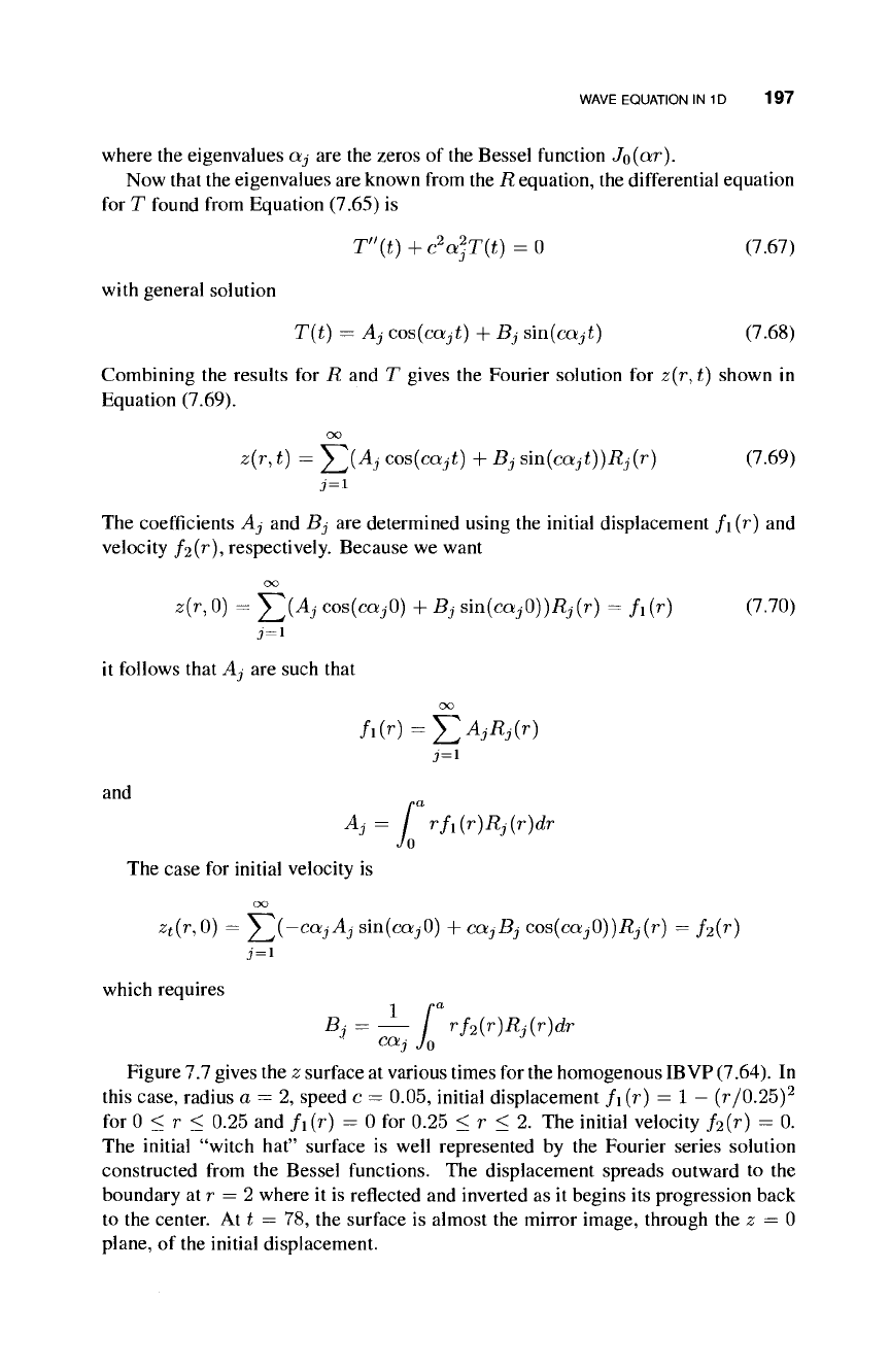
Figure 7.7 gives the z surface at various times for the homogenous IBVP

(7.64).

this case, radius a — 2, speed c = 0.05, initial displacement /i(r) = 1

—

(r/0.25)

for 0 < r < 0.25 and /i(r) = 0 for 0.25 < r < 2. The initial velocity /

(r) = 0.

The initial "witch hat" surface is well represented by the Fourier series solution

constructed from the Bessel functions. The displacement spreads outward to the

boundary at r = 2 where it is reflected and inverted as it begins its progression back

to the center. At t = 78, the surface is almost the mirror image, through the z = 0

plane, of the initial displacement.

198

WAVE EQUATION

Figure 7.7 Plots of z(r, t) for various values of t.

WAVE EQUATION IN 2D 199

7.2 WAVE EQUATION IN 2D

The wave equation in two spatial dimensions is shown in Equation (7.71). The

derivation is left

exercise.

The dependent variable z represents the displacement,

at a given location (x, y) and time ¿, of a surface from some reference level taken to

correspond to z = 0.

(x,

y, t) = c

(x, y, t) + z

(x, y, t)] + F(x, y, t)

(7.71)

A well-posed IBVP for z on a finite rectangular domain {(x, y)\0 < x < L and 0 <

y < M} for t > 0 require boundary conditions for z at x = 0, x = L, ?/ = 0, and

= M, as well as initial conditions for z and z

. The general form of an IBVP for a

two-dimensional elastic membrane is outlined in IBVP (7.72).

( ztt(x, y, t) = c

z{x, y, t) + F(x, y, t)

0<x<L, 0<y<M, t>0

IBVP<

z(x,y,0)

^t(^2/,0)

/i(^y)

aiZy(x,0,t) + biz(x,0,t) = gi(x,t)

(L, y, i) + &2^(^,

2/,

0 =

P2Í2/,

azZy(x, M, i) +

z(x,

M, i) = 03

(x,

^χ

(0,

y, í) + 6

2;(0,

j/,

t) = ^

(y, t)

(PDE)

(ICI)

(IC2)

(BC1)

(BC2)

(BC3)

(BC4)

(7.72)

The solution procedure for the 2D elastic wave is like that for the other IBVPs we

have already considered. We begin with the homogenous case for which the methods

of separation of variables and Fourier series provide a solution.

7.2.1 2D Homogeneous Solution

The homogeneous form of IBVP (7.72) results when F and gi{i = 1..4) are all

identically zero. We assume a solution of the form

z(x,y,t) = X(x)Y(y)T(t)

and when it is substituted into the homogeneous form of Equation (7.71), the equation

T"(t) X"(x) , Y"(y)

<?T{t) X(x)

Y(y)

-A

(7.73)

results after division by X(x)Y(y)T(t). As before, the separation constant —λ is

introduced. To allow for the separation of functions X and Y, the constant λ is

written as μ + v. The three ODEs shown in Equations (7.74) - (7.76) result.

Χ"(χ)+μΧ(χ) = 0

Y"{y) + uY{y) = 0

T"(t) + c

(ß + v)T(t) = 0

(7.74)

(7.75)

(7.76)

200

WAVE EQUATION

When Equation (7.74) is combined with BCs (BC2) and (BC4), a regular Sturm-

Liouville problem results for which properties

- 5 of Chapter 3 hold. The same is

true for Equation (7.75) in combination with BCs (BC1), and (BC3). Consequently,

we will let

X(a

x) and μ

—

n = 0,1,2,... (7.77)

represent the eigenfunctions and eigenvalues, respectively, for X. Similarly,

Y(ß

x) and v

= ß

0,1,2,...

(7.78)

will represent the eigenf unctions and eigenvalues, respectively, for Y.

With solutions for X and Y determined, the ODE in Equation (7.76) is considered

next. Both μ and v are non-negative. Both are zero only if bi(i — 1..4) are zero.

For most applications, one or both of μ or v is positive, so the general solution to

Equation (7.76) is

(t)

= Acos{c^/al+ßlt) + Bsm(cy/a

+ßlt)

Combining the results for the three separated ODEs gives

oo oo

z(x,y,t) = ΣΣ(

(7.79)

cos(cy/al + ßlfj

sm{c^/al + ß^tj X

x)Y

{ß

n=0 m=0

(7.80)

IBVP<

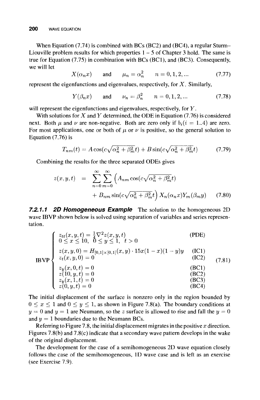
7.2.1.1

2D Homogeneous Example The solution to the homogeneous 2D

wave IBVP shown below is solved using separation of variables and series represen-

tation.

(x,y,t) = {V?z(x,y,t) (PDE)

0<x<10, 0 < y < 1, ¿>0

z(x,y,0) = i/[o,i]x[o,i]fo2/) · 15x(l -x)(l - y)y (ICI)

zt(x,y,0) = 0 (IC2)

(7e81)

(x,0,t)=0 (BCl)

¿(10,2/,i) = 0 (BC2)

Zy(x,l,t)=0 (BC3)

z(0,y,t) = 0 (BC4)

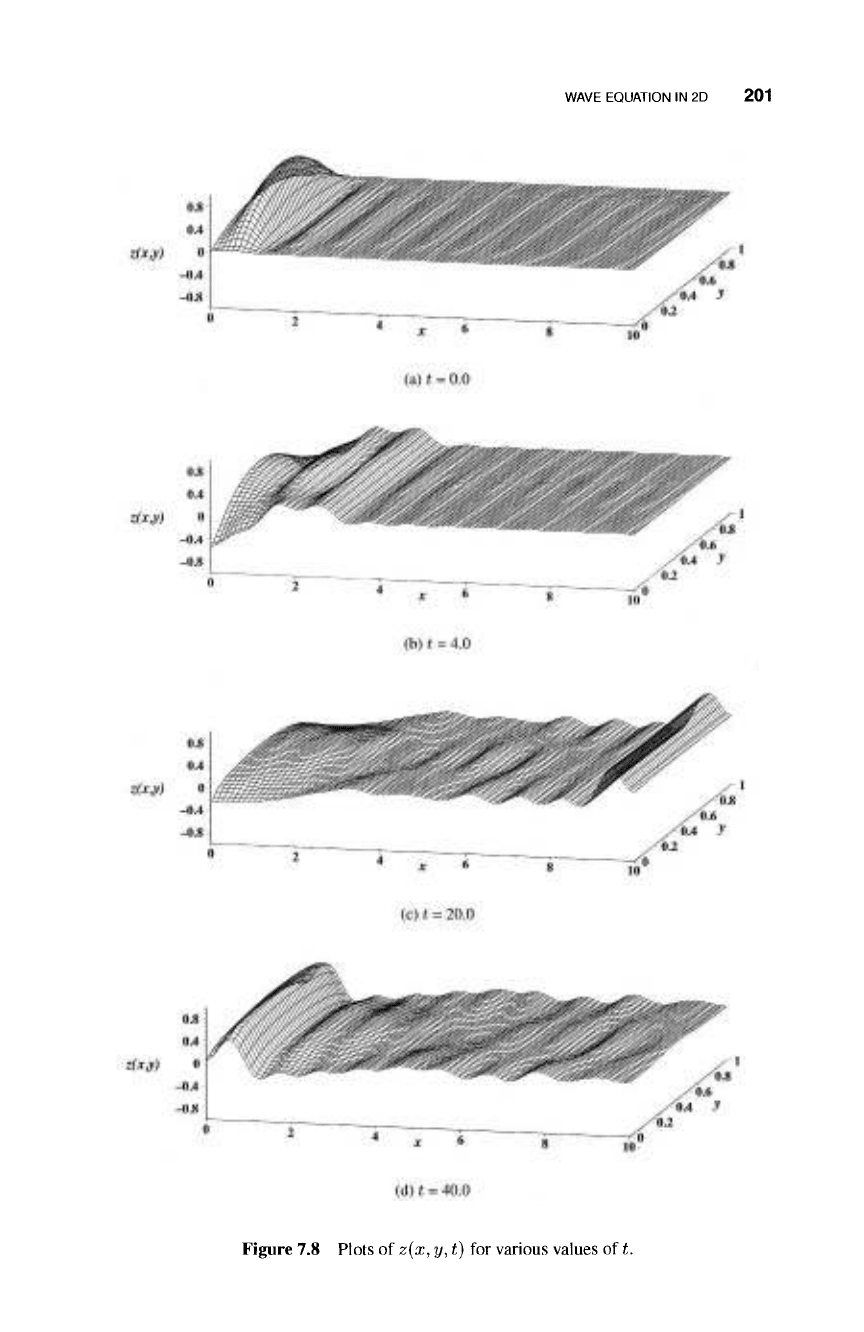
The initial displacement of the surface is nonzero only in the region bounded by

0 < x < 1 and 0 < y < 1, as shown in Figure 7.8(a). The boundary conditions at

y = 0 and y = 1 are Neumann, so the z surface is allowed to rise and fall the y = 0

and y

—

I boundaries due to the Neumann BCs.

Referring

Figure

7.8,

the initial displacement migrates in the positive x direction.

Figures

7.8(b)

and

7.8(c)

indicate that a secondary wave pattern develops in the wake

of the original displacement.

The development for the case of a semihomogeneous 2D wave equation closely

follows the case of the semihomogeneous, ID wave case and is left as an exercise

(see Exercise 7.9).

WAVE EQUATION IN 2D 201

Figure 7.8 Plots of z(x, y, t) for various values of t.