Bernatz R. Fourier Series and Numerical Methods for Partial Differential Equations

Подождите немного. Документ загружается.

202 WAVE EQUATION

EXERCISES

7.1 Solve the following IBVP using the method of d'Alembert. Use Maple to plot

the wave solution for t

0 and t = 2.

f ytt(x,t)=y

(x,t) (PDE)

-oo < x < oo, t > 0

IVP

2/t(M) = 0

(ICI)

(IC2)

IVP

(x,

t) =

(x,

t) (PDE)

—oo < x < oo, t > 0

î/(*>°) = W

2/t(*,0) = 0

(ICI)

(IC2)

7.2 Use the method of d'Alembert to solve the following IVP for the infinite string.

[

{x,t)

(x,t) (PDE)

—oo < x < oo, t > 0

IVP

2/(χ,0) = /(χ)

I Vt(x,0) =g(x)

(ICI)

(IC2)

1 1 /*

Answer: 2/(ar, t) = - [f(x - ct) + f(x + ct)} + — /

5(0^

7.3 Solve the following IBVP using the method of d'Alembert as derived in Exer-

cise 7.2. Use Maple to plot the wave solution for t

0 and t = 2.

(x,t)

(x,t) (PDE)

—oo < x < oo, í > 0

IVP

y(x,0) = 0

Vt(x,0) = f^

(x,t)

—oo < x < oo, í > 0

y(z,o) = i^

(ici)

(IC2)

(PDE)

(ICI)

(IC2)

7.4 Solve the following homogeneous IBVP using Fourier series methods. In each

case (i) specify the eigenvalues and eigenfunctions, (ii) provide a plot of the Fourier

partial sum (at least 30 terms) approximation to non-zero initial displacement or

velocity (both if so required), (iii) provide a plot of the displacement for t = 5, and

(iv) state the value of 2/(5,1).

EXERCISES

203

IBVP^

( ytt(x,t)

(x,t)

0 < x < 10, t > 0

y(x,0)

[4>6]

(x)(4

- x)(x

t/t(x,0)

= 0

y(0,t)

= 0

y(10,t)=0

IBVP¿

yttjx, t) =Jy

10, t > 0

2/(0,i)=0

(W,t)

= 0

m{x,t) = 3y

(x,t)

3 < x < 10, t > 0

y(0,t)

= 0

y(l0,t)

= 0

(PDE)

(ICI)

(IC2)

(BC1)

(BC2)

(PDE)

y(x,o)

(ici)

(x,

iï

(x) (4

x) (x

- 6) (IC2)

(BC1)

(BC2)

(PDE)

y(x,0) =x(10-x)/50

(ICI)

(x,0)

Η[

,β](χ)(4

- x)(x - 6) (IC2)

(BCD

(BC2)

7.5 Solve

the

following semihomogeneous IBVP using Fourier series

(at

least

terms) methods. For each, (i) specify the eigenvalues and eigenfunctions, (ii) provide

a plot

the displacement

for t - 5, and

(iii) state the value

y(5,1).

(x,t)

F*(x,t)

(PDE)

< x < 10, t > 0

IBVP ·{

!/(x,0)

= 0 (ICI)

îfc(x,0)=0

(IC2)

y(0,t)=0

(BC1)

I y(10,t)=0 (BC2)

F*(x,t) = (x - 4.5)(5.5 - x)//

[

,5.5](x)e-

f Wx,i) = 2y

(x,t) + F*(x,t) (PDE)

0 < x < 10, t > 0

TRVP/ 2/(

'°)

1^(10-χ)

1 î/t(x,0)

= 0

y(o,í) = o

l y(10,í)=0

(ici)

(IC2)

(BCl)

(BC2)

204

WAVE EQUATION

= 4(x -

2)(3

x)if

](x) sin*

- 4(x -

7)(8

x)H

¿](x) siní

7.6 Solve

the

following nonhomogeneous IBVP using Fourier

(at

least

terms)

series methods. For each,

(i)

specify the eigenvalues and eigenfunctions, (ii) provide

a plot

of the

displacement

for t = 5, and (iii)

state

the

value

y(5,1).

Assume

y(x,t)

Y(x,t)

S(x,t),

where S(x,t)

= A(t) +

B(t)x. Specify

the

formulas

for

A(t)

and

B(t).

IBVP<

ytt(x,t)

< x < 10, t > 0

2/(x,0)=0

îfe(*,0)=0

y(o,t)

= e-*

2/(10,i)

= 0

(x,¿)

(PDE)

(ICI)

(IC2)

(BCl)

(BC2)

IBVP<

ytt[x,t)

{x,t)

(PDE)

< x < 10, ¿ > 0

2/(x, 0)

ίΤ

[4ϊ6

](χ)(4

- *)(x - 6) (ICI)

2/t(*,0)

= 0 (IC2)

(0,£)=0

(BCl)

2/(10,

í) =

sint

(BC2)

7.7 Solve the following 2D homogeneous IBVPs using Fourier series methods

(at

least 30 terms). For each, (i) specify the eigenvalues and eigenfunctions, (ii) provide

a plot

the displacement

for t

and (iii) state the value

of z(b,

5,5).

Ztt(x,y,t)

z(x,y,t)

(PDE)

< x < 10, 0 < y < 10, t > 0

2(x,î/,0)

,6]x

[4,6]

(*,!/)(*

4)(6

- x)(y -

4)(6

- y) (ICI)

zt(x,y,0)

= 0 (IC2)

(x,0,t)

= 0 (BCl)

2(10,y,f)=0

(BC2)

(x,10,t)

=0 (BC3)

^(0,í/,í)

= 0 (BC4)

IBVP<

(x,y,t)

z(x,y,t)

(PDE)

< x < 10, 0 < y < 10, t > 0

*(*,y,0)=0

(ICI)

ZÉ(X,2/,0)

= #[

,6]χ[4,6](*,2/)(* - 4)(6 - x)(y - 4)(6 - y) (IC2)

(x,0,t)

= 0 (BCl)

4l0,î/,i)=0

(BC2)

(x, 10,

t) =0 (BC3)

*(0,î/,i)

= 0 (BC4)

EXERCISES 205

IBVP<

(x,y,t) = 2V

z{x,y,t) (PDE)

0 < x < 20, 0 < y < 10, t > 0

*(x,2/,0) = H

mxm

(x,y)(x - 4)(6 - x)fo - 4)(6 - y) (ICI)

zt(x,y,0) = 0 (IC2)

(BC1)

(BC2)

(BC3)

(BC4)

Zy(X,0,t) = 0

foo,y,t) =0

(x,10,t) =0

[ z(0,î/,t) = 0

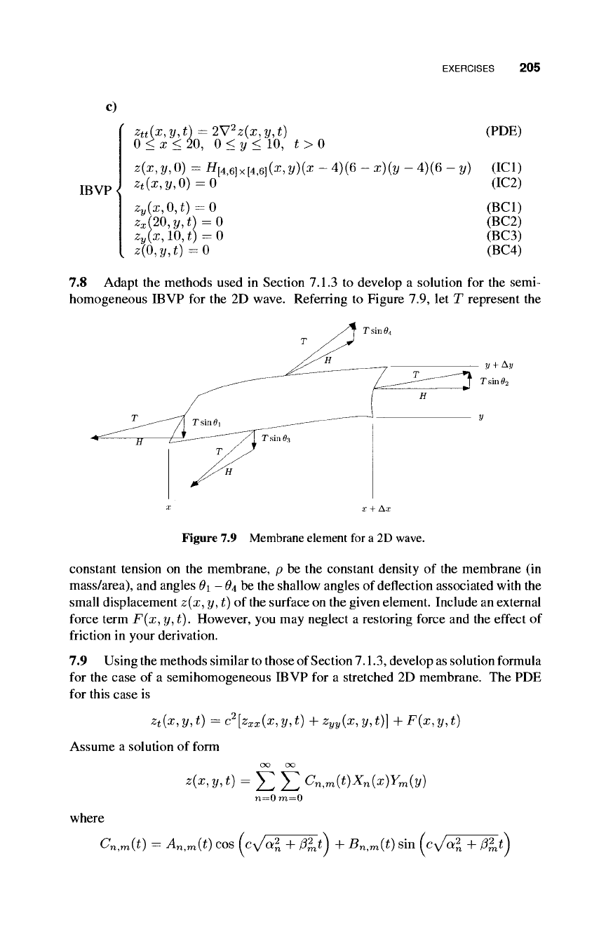
7.8 Adapt the methods used in Section 7.1.3 to develop a solution for the semi-

homogeneous IBVP for the 2D wave. Referring to Figure 7.9, let T represent the

x x

Figure 7.9 Membrane element for

2D wave.

constant tension on the membrane, p be the constant density of the membrane (in

mass/area), and angles θ\ -

θ±

be the shallow angles of deflection associated with the

small displacement z(x, y, t) of

the

surface on the given element. Include an external

force term F(x,y,i). However, you may neglect a restoring force and the effect of

friction in your derivation.

7.9 Using the methods similar

those of Section

7.1.3,

develop as solution formula

for the case of a semihomogeneous IBVP for a stretched 2D membrane. The PDE

for this case is

{x,y,t) =c

(x,y

t) + z

(x,y,t)] + F{x,y,t)

Assume a solution of form

where

Z{x,y,t) = ΣΣ Cn,m{t)Xn(x)Ym(y)

n=0 ra=0

,m(t)

= A

(t) COS [C^/al + ßlS) +

n,m(t) SHI \Cy/a\ + ß^tj

206

WAVE EQUATION

The process should result in

,m\t)

-sin [cy/a^ + ß^t) F

m(t)

and

Β'η,τηίϊ)

W (sin (cy/al + fai) ,cos (cy/a*+fat))

COS

[Cy/ofa + ß^t) F

(í)

W (sin (cy^T^i) ,cos (cy/al + fat))

7.10 Solve the following IBVP in polar coordinates with /i(r) = 0 and /2ΟΌ =

1 - (r/0.25)

for 0 < r < 0.25 and ^(r) = 0 for 0.25 < r < 2. Plot the z(r, </>,£)

surface for the same times as those in Figure 7.7 as a means of comparing the two

results.

( z

(r, t) = c

(r, t) + ±z

(r, t)) (PDE)

0 < r < a, t > 0

IBVP<

*(r,0) = /i(r)

**(r,0)=/

(r)

z(a,i) = 0

|2/(r,i)|

< 00

(ICI)

(IC2)

(BCl)

(BC2)

(7.82)

CHAPTER 8

NUMERICAL METHODS: AN OVERVIEW

The PDEs associated with most science and engineering applications are often impos-

sible,

or impractical, to solve using analytic methods, such as separation of variables

and Fourier series. Numerical solution methods provide a reasonable alternative

in many of these situations. The purpose of this chapter is to provide a general,

brief overview of numerical methods. Common features and terminology associated

with many of the various numerical methods are introduced, as well as the basic

fundamental principals of three such methods.

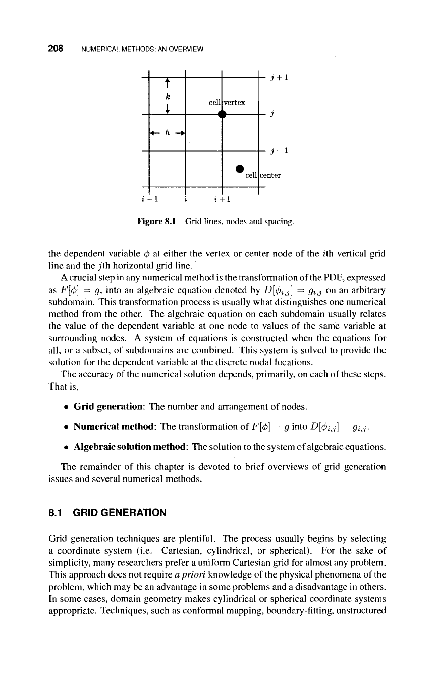
Numerical methods typically begin by dividing, or discretizing, the problem

domain into a number of small subdomains, or elements, defined by grid lines.

Dependent variable values are determined for a finite number of domain locations

called grid points, mesh points, or nodes. Nodes located at the intersection of grid

lines are called cell vertex nodes, while those located inside the elements defined

by the grid lines are classified as cell center nodes, as indicated in Figure 8.1. The

distance between consecutive grid lines is called the grid spacing, denoted by "/i"

and "fc" in Figure

8.1.

The spacing is said to be uniform in the horizontal direction if

h is constant, and uniform in the vertical direction if k is constant. If h

—

k, the grid

is said to be square. The grid lines and associated nodes are referenced by indices

such as "i" and

"j"

shown in Figure 8.1. Consequently, φι^ represents the value of

Fourier Series and Numerical Methods for Partial Differential Equations, 207

First Edition. By Richard Bernatz

208 NUMERICAL METHODS: AN OVERVIEW

L-

h -*

cell vertex

cell

—

+ 1

Figure

8.1

Grid lines, nodes and spacing.

the dependent variable

φ at

either the vertex

center node

the

úh

vertical grid

line and the

j\h

horizontal grid line.

A crucial step in any numerical method is the transformation of the

PDE,

expressed

as F[</>]

= g,

into

algebraic equation denoted

by Ό[φ^]

—

gi¿ on an

arbitrary

subdomain. This transformation process is usually what distinguishes one numerical

method from

the

other. The algebraic equation

each subdomain usually relates

the value

the dependent variable

at one

node

values

the same variable

surrounding nodes.

system

equations

constructed when

the

equations

for

all,

or a

subset,

subdomains are combined. This system

solved

provide

the

solution

for

the dependent variable

the discrete nodal locations.

The accuracy of

the

numerical solution depends, primarily, on each of these steps.

That is,

• Grid generation: The number and arrangement

nodes.

• Numerical method: The transformation

F[</>]

= g

into Dfyij]

= gij.

• Algebraic solution

method:

The solution to the system of algebraic equations.

The remainder

this chapter

devoted

brief overviews

grid generation

issues and several numerical methods.

8.1 GRID GENERATION

Grid generation techniques

are

plentiful. The process usually begins

selecting

a coordinate system

(i.e.

Cartesian, cylindrical,

spherical).

For the

sake

simplicity, many researchers prefer a uniform Cartesian grid for almost any problem.

This approach does not require a priori knowledge

the physical phenomena of the

problem, which may be an advantage in some problems and a disadvantage in others.

In some cases, domain geometry makes cylindrical

spherical coordinate systems

appropriate. Techniques, such as conformai mapping, boundary-fitting, unstructured

GRID GENERATION 209

grids,

multigrids, or adaptive

grids,

may be used for "irregular" geometries or complex

flow characteristics as well.

A key objective in many grid generation efforts is to assure a boundary in the

computational domain corresponds to a boundary in the physical domain. This goal

may be referred to as geometric adaptation. Additionally, it may be desired to

include greater nodal resolution in the physical domain where a dependent variable

changes quickly. This process may be referred to as solution adaptation. It may

be desirable to increase grid resolution in regions where a dependent variable has a

large gradient change during the solution process. The steep-gradient region(s) may

change location as the solution evolves. Grid processes that change grid resolution

may be referred to as automatic or dynamic solution adaptation. This technique

may be useful, for example, in the case of

moving internal boundary corresponding

to a phase change.

The computational grid should be constructed with the following objectives:

A. Minimize numerical error. Grid resolution and orientation with respect to

flow direction may impact sources of numerical error, such as round-off and

truncation error.

Provide numerical stability. The stability (to be discussed later) of some

numerical methods depends on the size of the discretization element.

C. Provide computational economy. Obviously, more computation is required as

the number of grid nodes increases.

Provide ease in handling boundary conditions. Boundary conditions may

involve normal derivatives in some applications. Consequently, it is advanta-

geous for certain grid lines to adjoin the boundary in a normal fashion.

Some objectives in the list above are at odds with each other. For example,

objective C suggests the need for fewer nodes while objectives A and B seem to

require more nodes. Indeed, the tension between too few and too many nodes is often

at the center of the grid generation issue. The overall objective is the optimal grid;

the most sparse grid system that provides the desired accuracy.

The principles outlined below may be used to attain one or more of the stated

objectives. The objectives addressed by a given principle are listed in parentheses.

The problem geometry aligns with the coordinate system. (A, C, and D)

Flow and heat flux vectors should run parallel to the coordinate lines. (A)

In the case of nonuniform grid spacing, the ratio (larger to smaller) of spacing

for two adjacent cells should be < 2. (A and B)

The coordinate system should be orthogonal or nearly orthogonal whenever

possible. (A and B)

Node density should be proportional to the gradient of a dependent variable.

(A and B)

210 NUMERICAL METHODS: AN OVERVIEW

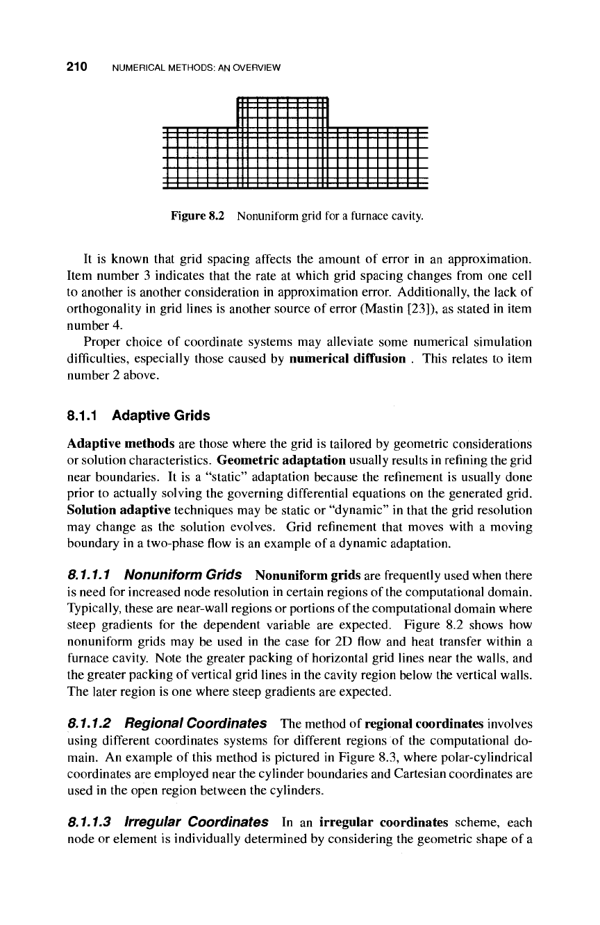
Figure 8.2 Nonuniform grid for

furnace cavity.

It is known that grid spacing affects the amount of error in an approximation.

Item number 3 indicates that the rate at which grid spacing changes from one cell

to another is another consideration in approximation error. Additionally, the lack of

orthogonality in grid lines is another source of error (Mastín [23]), as stated in item

number 4.

Proper choice of coordinate systems may alleviate some numerical simulation

difficulties, especially those caused by numerical diffusion . This relates to item

number 2 above.

8.1.1 Adaptive Grids

Adaptive methods are those where the grid is tailored by geometric considerations

or solution characteristics. Geometric adaptation usually results in refining the grid

near boundaries. It is a "static" adaptation because the refinement is usually done

prior to actually solving the governing differential equations on the generated grid.

Solution adaptive techniques may be static or "dynamic" in that the grid resolution

may change as the solution evolves. Grid refinement that moves with a moving

boundary in a two-phase flow is an example of a dynamic adaptation.

8.1.

Nonuniform Grids Nonuniform grids are frequently used when there

is need for increased node resolution in certain regions of the computational domain.

Typically, these are near-wall regions or portions of the computational domain where

steep gradients for the dependent variable are expected. Figure 8.2 shows how

nonuniform grids may be used in the case for 2D flow and heat transfer within a

furnace cavity. Note the greater packing of horizontal grid lines near the walls, and

the greater packing of vertical grid lines in the cavity region below the vertical walls.

The later region is one where steep gradients are expected.

8.1.1.2 Regional Coordinates The method of regional coordinates involves

using different coordinates systems for different regions of the computational do-

main. An example of this method is pictured in Figure 8.3, where polar-cylindrical

coordinates are employed near the cylinder boundaries and Cartesian coordinates are

used in the open region between the cylinders.

8.1.1.3 Irregular Coordinates In an irregular coordinates scheme, each

node or element is individually determined by considering the geometric shape of a

GRID GENERATION 211

Figure 8.3 Regional coordinates for

flow

between cylinders.

Figure 8.4 Irregular coordinates for

flow

around a cylinder.

boundary. It is frequently used in finite element methods. In this case, the triangu-

lar shape of the cell allows for easier alignment with irregular boundaries. Figure

8.4 indicates how the irregular placement of nodes, and the corresponding elements

created by the nodes, makes for a fair approximation of a circular boundary.

8.1.1.4

Solution Adaptation The Seabreeze circulation associated with

land-

water interface, such as a sea coast, is a situation in which a solution adaptive grid

may be used. The difference in surface temperatures between the land and water

creates an on-shore flow of cool and moist air. The flow begins at the land-water

boundary and moves inland creating a "front," where an abrupt change in wind speed,

air temperature and humidity occur. It is important to refine the grid near the front

to simulate and investigate the dynamics of this phenomenon. It is more efficient

to limit the resolution to the frontal area instead of applying the required resolution

unnecessarily to the entire domain.

Figure 8.5 shows the "dynamic" local grid resolution move through the domain

with the location of the sea breeze front.

calculation of dependent variable gradients