Bernatz R. Fourier Series and Numerical Methods for Partial Differential Equations

Подождите немного. Документ загружается.

262 FINITE ELEMENT METHOD

as that by Johnson [18] or that by Mitchell and Wait [25]. The discussion presented

here is limited to the case of elliptic ID and 2D boundary value problems. For the

sake of easier reference, three related problems will be restated next.

The first is the original boundary value problem on the bounded, open domain Ω.

That is,

( Du = f (PDE)

BVP^

(10.21)

I u\an = 9 (BC)

where D is an elliptic differential operator on the set V of admissible functions. The

weak reformulation of BVP (10.21) is: find ueV, such that

a(u,v) = (/,v) VveV (10.22)

The Galerkin approximation to Equation (10.22) is: find Uh

V^, such that

o(u

,v) = (/,v)

VVGV^

(10.23)

The following theorem is stated without

proof.

Theorem 10.1 Let u be the solution to Equation (10.22) and Uh be the solution to

(10.23).

Then there exist a positive constant C, such that

||u-u

||v<C||u-v||v

for all v

V^.

The norm || · ||y is based on a bilinear form defined on the space V. The first remark

relative to the theorem is that, of all the elements v of V/¿, Uh provides the best

approximation for u. Further, an upper bound for the distance between Uh and u

may be determined by selecting any single function v of V^.

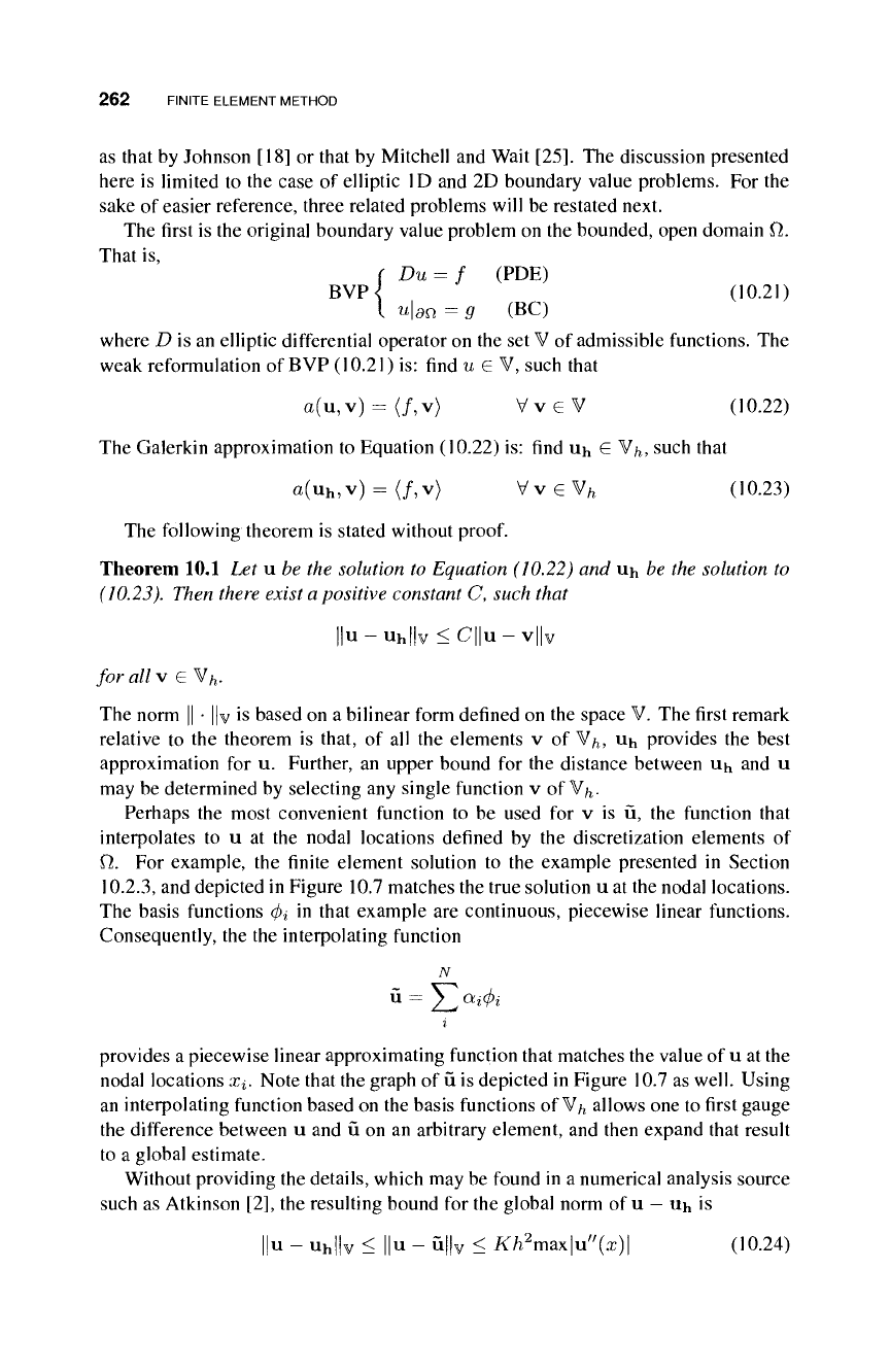
Perhaps the most convenient function to be used for v is u, the function that

interpolates to u at the nodal locations defined by the discretization elements of

Ω. For example, the finite element solution to the example presented in Section

10.2.3,

and depicted in Figure 10.7 matches the true solution u at the nodal locations.

The basis functions φι in that example are continuous, piecewise linear functions.

Consequently, the the interpolating function

= Σ

OLi

provides a piecewise linear approximating function that matches the value of u at the

nodal locations x¿. Note that the graph of ü is depicted in Figure 10.7 as well. Using

an interpolating function based on the basis functions of V^ allows one to first gauge

the difference between u and ü on an arbitrary element, and then expand that result

to a global estimate.

Without providing the details, which may be found in a numerical analysis source

such as Atkinson [2], the resulting bound for the global norm of u

—

Uh is

||u - UhHv < ||u - u||v < Ä7i

max|u"(x)| (10.24)

ERROR ANALYSIS 263

0.15

0.05

Figure 10.7 True solution u and the linear interpolation function ü.

where h is the length of the (uniform) grid spacing, K is an unknown positive

constant, and the maximum absolute value of the second derivative of u is taken over

the entire interval 0 < x < 1. The conclusion drawn from this result is that the

finite element solution constructed from piecewise linear basis functions has a global

truncation error on the order of h

. The length h is either the uniform node spacing,

or the maximum node spacing in the case nonuniform spacing is used. Additionally,

the finite element approximation u^ converges to the true solution u as h tends to

zero provided the second derivative of u is bounded.

The results above may be shown to be true for the more general case of an elliptic

operator D on a 2D open, bounded domain Ω. That is, if the finite element solution

u^ is found using subspace V^ of piecewise linear functions, then there exists a real

number K such that

—

uJ|v < Kh max

dx\)

\dx

1/2

(10.25)

where the maximum is taken over the entire domain Ω. In the 2D case, the value

used for h is the largest length of any line connecting nodes of a given element.

Further, if the subspace V^ of V is comprised of piecewise polynomials of degree

r > 1, then the result given in Inequality (10.25) generalizes to

|u-u^||

<i^/i

r+1

max

r+1

δχγ

r+1

dxY

:-|l/2

(10.26)

264 FINITE ELEMENT METHOD

10.5 1D PARABOLIC EXAMPLE

Finite element methods for solving a 1D, nonhomogeneous heat equation IBVP are

described in the section. The weak form of the IBVP is developed in a way very

similar to the steady-state case. An approximate solution to the weak formulation is

identified from the finite dimensional subspace of functions that are piecewise linear

on the finite elements of the problem domain. However, the weights needed for

expressing the approximate solution as a combination of basis functions must vary

in time because the solution varies in time. How the time-dependency is included in

the solution process is one distinguishing feature of various finite element methods

for this class of

problems.

Two such means methods will be described in the material

of this section. A statement of the IBVP and its weak formulation are given next.

10.5.1 Weak Formulation

The IBVP is

( u

—

(x, t) = q{x,

£),

a < x <b, t > 0 (PDE)

u(x, 0) = /(x), a < x < b (IC) (io.27)

IBVP<

u(a,t)=0, t>0 (BCl)

t u(b,t) -0, t >0 (BC2)

The solution u is from the set V of functions differentiate in ¿, for t > 0 and twice

differentiate in x, for a < x < b. The weak form of the PDE in IBVP (10.27) is

v) + ka(u, v) = (q, v) (10.28)

where

rb pb

I u

(x,t)v(x,t)dx (f,v) = / q(x,t)v(x,t)da

Ja Ja

and

pb nb

a(u,v) =

—

/ u

{x,t)v(x,t)dx = / u

{x,t)v

{x,i)di

Ja Ja

The set Vh is the subspace of V consisting of continuous functions that are

piecewise linear on the uniform elements that partition the interval [a,

as defined

in Section

10.2.3.

As in the previous case, a basis for

is the set {0i, 02, · · ·,

</>m}>

such that

(j>i(xj)

— lfoxi=j and 0 otherwise. The points Xj represent the nodes of

the discretization of [a,

b].

The finite element solution from Vh has the form

(x,t)

y]vi(t)<i>i(x)

i=l

and substitution in Equation (10.28) gives

Mrf(t) + kKrf(t) = b(t) (10.29)

1D PARABOLIC EXAMPLE

265

where

and

= /

φι{χ)φ

{χ)άχ

Kij = /

φ\{χ)φ^{χ)άχ

bi(t)

= /

ς(χ,ί)φ

(χ)άχ

Equation (10.29) offers

semidiscretization

Equation (10.28)

that no time

discretization is employed. Section 10.5.2 presents the method of lines in which

Equation (10.29)

integrated with respect to time resulting in

formula for the

time-dependent vector f}(t) in terms of the other quantities.

10.5.2 Method of Lines

The matrix

in Equation (10.29) is tridiagonal and invertible with inverse repre-

sented by

Multiplying both sides of the equation by M"

gives

ff(t)+Af¡(t)=g(t)

(10.30)

where

kM~

and

g(t) = M~

b{t)

Equation (10.30) is a system of linear, nonhomogeneous ODEs that may be solved,

in a way similar to a single ODE, using the integrating factor

It is left as an exercise (see Exercise 10.7) to show that

*ψ-

= BA

(10.31)

The result for if(t) using the integrating factor A(i) is

where

ff(t)

rf(0)

+ /

g(s)ds (10.32)

η%(0)

= /

ς{χ,0)φ

(χ)άχ

Although Equation (10.32) provides a formula for the weights

ff(t),

the practicality

of the formula is in question because, among other reasons, the matrix

is not sparse

because

is formed using the inverse of M, which is not sparse. Another means

for determining the finite element approximation to the solution of IBVP (10.27) is

described in Section

10.5.3.

266 FINITE ELEMENT METHOD

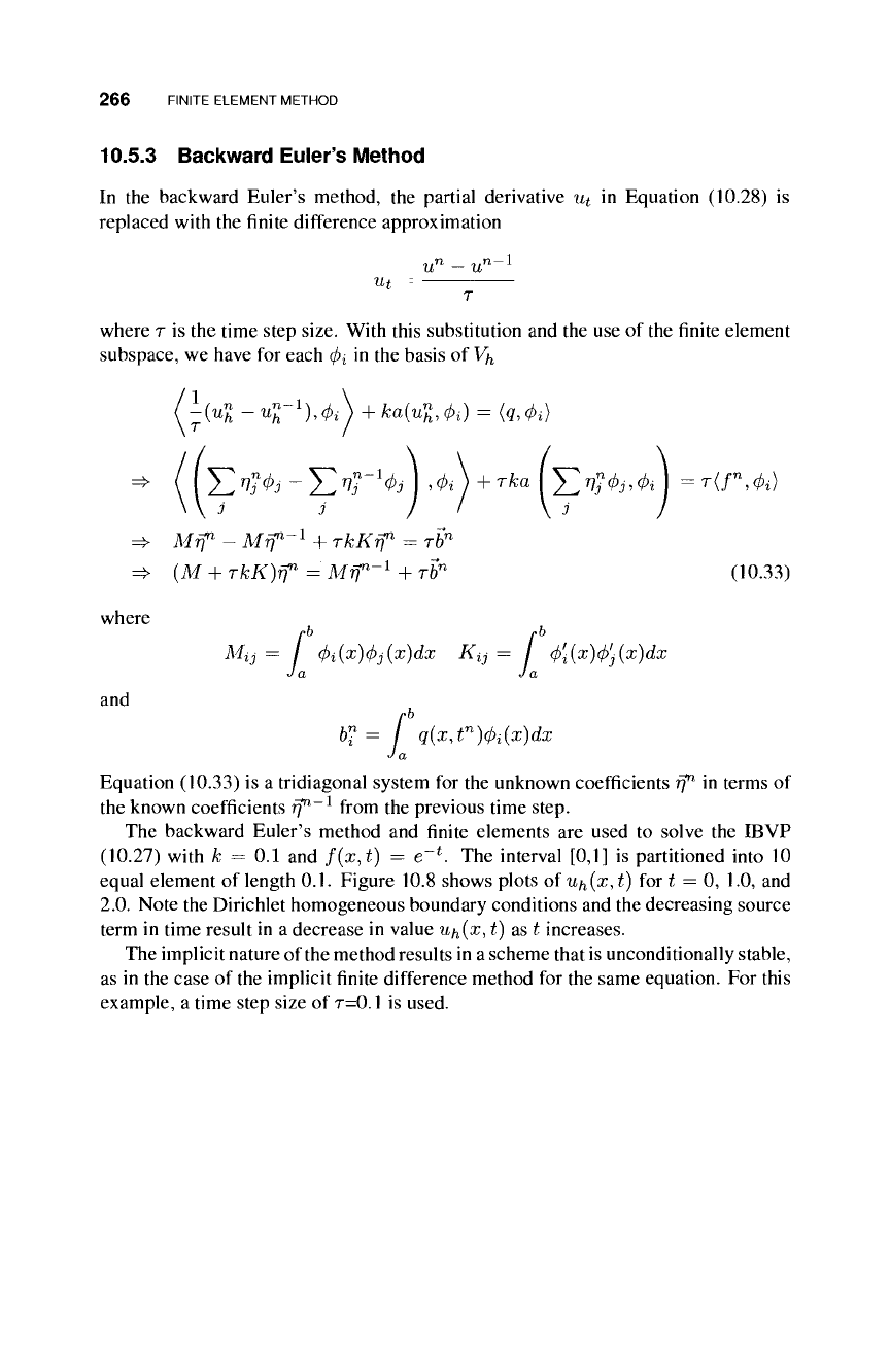
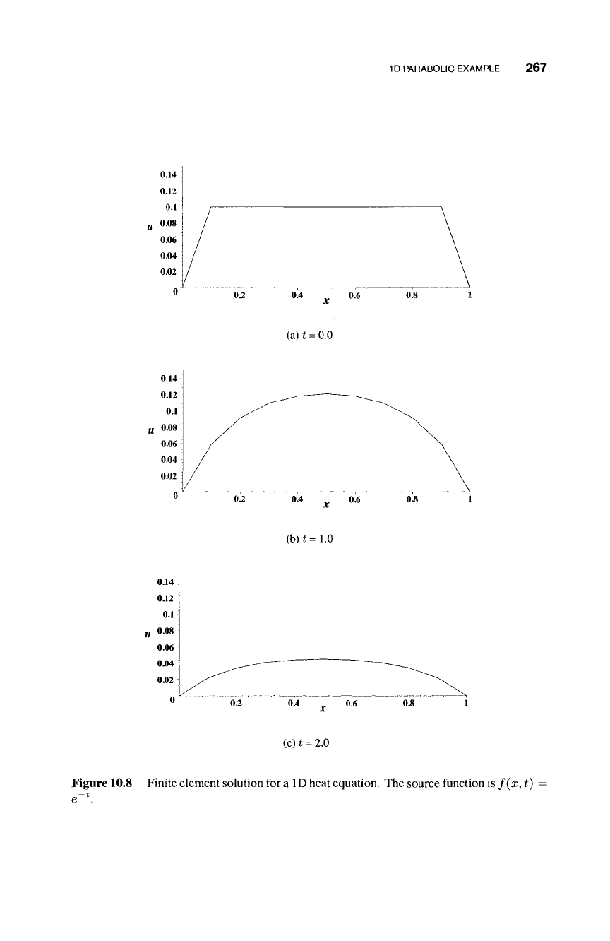
10.5.3 Backward Euler's Method

In the backward Euler's method, the partial derivative u

in Equation (10.28) is

replaced with the finite difference approximation

n _

n-l

where r is the time step size. With this substitution and the use of the finite element

subspace, we have for each φ

in the basis of

(l« -η^,φλ

+ka{u

,4>i)

(q,4>i)

Wi - Σ

-1

)

></>*)+

Tka

(

Σ ^

& ) =

> &>

=Φ-

Mff

- Mrp-

TkKff

= rb

=*■ (M + TkK)fT =

Mff

+ rb

(10.33)

where

¡>b pb

Mij = / 4)i{x)(¡)j{x)dx Kij = / φ[{χ)φ^{χ)άχ

Ja Ja

b?= í q(x,t

)4>i(x)dx

Equation (10.33) is a tridiagonal system for the unknown coefficients rf

in terms of

the known coefficients rf

1-1

from the previous time step.

The backward Euler's method and finite elements are used to solve the IBVP

(10.27) with k = 0.1 and f(x,t) = e~

. The interval [0,1] is partitioned into 10

equal element of length 0.1. Figure 10.8 shows plots of Uh(x, t) for t

—

0, 1.0, and

2.0.

Note the Dirichlet homogeneous boundary conditions and the decreasing source

term in time result in a decrease in value w^(x, t) as t increases.

The implicit nature of the method results in a scheme that is unconditionally stable,

as in the case of the implicit finite difference method for the same equation. For this

example, a time step size of r=0.1 is used.

and

1D PARABOLIC EXAMPLE 267

0.14

0.12

0.1

0.08

0.06

0.04

0.02

0.4 0.6

0.8

(a)

0.0

(b)i=1.0

0.14

0.12

0.1

0.08

0.06

0.04

0.02

0.4 0.6

(c)

2.0

Figure 10.8 Finite element solution for a

heat equation. The source function is f(x, t)

-t

268 FINITE ELEMENT METHOD

EXERCISES

10.1 Provide details to show the following are equivalent expressions for the func-

tional

defined

Section

10.2.1

-(Dv,v)-(f,v) = ±(v

y)-(f,v)

10.2 Show, based

on the (i)

definition

the operator

A, (ii)

definition

(·,·),

and

the

boundary requirements

of u

and

v G V in

Section

10.2.1,

that (Au,v)

—

(f,v)^(v',u')

(f,v).

10.3 Provide details

show that

α^ =

for i =

a^=-10

for \i

—

= 1, and

dij

= 0 for

all other cases

the example presented

Section

10.2.3.

10.4 Verify the result given

for

b\ in Equation (10.15)

Section

10.2.3.

10.5 Consider the ID BVP

( -u"(x)

10x(l-x)

(DE)

BVP<^ (10.34)

[

u(0) =

-l,u(l)

= 2 (BC)

Use

the

linearity

the operator —d

/dx

and the

solution

BVP (10.13) given

in Section 10.2.3

determine

the

finite element solution

BVP (10.34) using

uniform elements.

10.6 Generalize the methods

for

a parabolic ID IBVP given in Section 10.5 to two

spacial dimensions.

10.7 Verify that the expression given

Equation

(10.31 )

is correct.

10.8 Provide the details on the integration process that results in the formula shown

in Equation (10.32).

10.9 This exercise pertains to the example presented in Section 10.2.3 and the error

bound given

Inequality (10.24).

a) Determine

the

value

K for

the solution found

Section

10.2.3.

Use

the

following definition

for || · ||

v(x)v(x)(¿£

b) Reduce

to 0.05 and calculate a bound on

||u

— Uh ||

using the value

of K

determined

part (a). Show that the bound determined

this way does,

indeed, provide

upper bound

for ||u

—

Uh||.

10.10 Verify that

a(u,v)

= / /

—V

u(x,y)v(x,y)dxdy=

/ /

Vu(x,y) -\7v(x,y) dxdy

Jn J Jn

EXERCISES 269

as stated in Section

10.3.1.

10.11 The purpose of this exercise is to provide development details for the stiffness

matrix used in Section 10.3.2. Let

be the isosceles right triangle with right angle at

the origin (0,0) and vertices at

(

1,0) and (0,1). Let ψι be the linear function on defined

Ω such that ^i(0,0) = 1, φι(1,0) = 0, and ^>i(0, 1) = 0, ^2 be the linear function

on defined Ω, such that ^i(0,0) = 0, ^i(l,0) = 1, and ^i(0,1) = 0, ψ

be the

linear function on defined Ω, such that φ\ (0,0) = 0, ^i(l,0) = 0, and^i(0,1) = l.

Define the stiffness matrix M to be such that M¿¿ = / /

νψι · Vtpj dxdy.

a) Show that

1 _I _I

1 2 2

-- - 0

2 y

-- 0 -

b) Use the result in part (a) to j ustify the resulting entries in the stiffness matrix

M given in Section 10.3.2.

10.12 Solve the following parabolic IBVP using finite element methods provided

in Section

10.5.3.

Use a uniform grid spacing of h = 0.1 and a time step size r = 0.1.

IBVP<

—

{x, t) = q(x, £), a < x < b, t > 0 (PDE)

u(x,0) = f(x), a<x<b (IC)

(10.35)

u(a,t) = 0, t>0

tfc(M)=0, t>0

(BC1)

(BC2)

a) a=0, 6=1, q(x,t) = x(l - x), f{x) = 0

b) a=0, 6=2, q(x, t) = x(2

—

x)e~

, f(x) = sin(7rx)

c) a=0, 6=1, q(x,t)

—

sin(7rx) cos

¿,

f(x) = 0

d) a=0, 6=2, q(x, t) = ^g^, f{x) = x(2 - x)

This Page Intentionally Left Blank

CHAPTER 11

FINITE ANALYTIC METHOD

The finite analytic (FA) method for the ID and 2D transport equations is presented

in this chapter. Because the transport equation for scalar quantities includes both

a convection term and a diffusion term, it is often referred to as a "convection-

diffusion" equation. The development of the FA method for the transport equations

is more general than that offered in previous chapters on the finite difference and

finite element methods. The resulting formulations reduce to the heat equation in ID

and 2D, as well as Poisson's and Laplace's equations in 2D.

The central concept of the FA method, introduced by Chen and Li [7], is the

use of separation of variables and Fourier series solutions on a locally linearized

version of the nonlinear convection-diffusion equation. Boundary conditions for each

FA element are constructed using the value of the dependent variable at the nodal

locations on the element boundary. Once the boundary functions are determined,

the Fourier series general solution is used to represent the boundary functions. The

Fourier coefficients determined in this process are expressed in terms of

the

boundary

nodal values, and a function for the dependent variable results. This function is

evaluated for the center of the element that gives the new value of the dependent

variable there in terms of the boundary node values. The coefficients for these nodal

locations are the finite analytic coefficients.

Fourier Series and Numerical Methods for Partial Differential Equations, 271

First Edition. By Richard Bernatz