Bernatz R. Fourier Series and Numerical Methods for Partial Differential Equations

Подождите немного. Документ загружается.

282 FINITE ANALYTIC METHOD

ΦΝ\¥

Φ"

<t>sw

ΦΝ(Χ)

-Φτ-

PNC ΨΝΕ

ΦΡ ΦΕΟ

ΦβΟ ΦβΕ

'(*)

Φ-Μ-

Φ- —

L—

h —4«— h —H

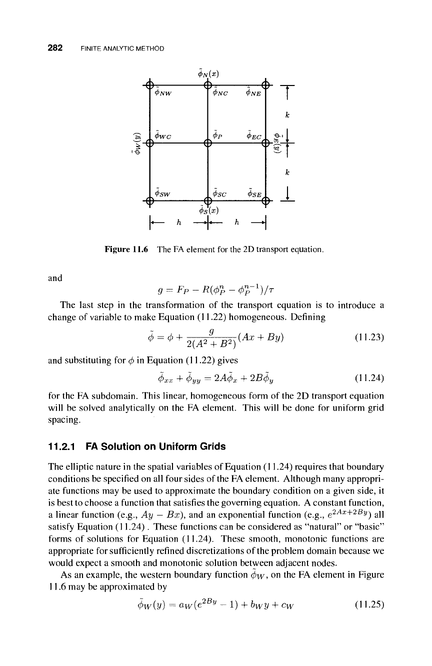
Figure 11.6 The FA element for the 2D transport equation.

and

g = F

-R(<t>

-<t>

)/r

The last step in the transformation of the transport equation is to introduce a

change of variable to make Equation (11.22) homogeneous. Defining

■

-(Ax + By)

2(A

+ B

)

and substituting for φ in Equation (11.22) gives

Φχχ -f

4>yy

= 2Αφ

2B(j)y

(11.23)

(11.24)

for the FA subdomain. This linear, homogeneous form of the 2D transport equation

will be solved analytically on the FA element. This will be done for uniform grid

spacing.

11.2.1 FA Solution on Uniform Grids

The elliptic nature in the spatial variables of Equation (11.24) requires that boundary

conditions be specified on all four sides of the FA element. Although many appropri-

ate functions may be used to approximate the boundary condition on a given side, it

is best to choose a function that satisfies the governing equation. A constant function,

a linear function (e.g., Ay

—

Bx), and an exponential function (e.g.,

2Ax

satisfy Equation (11.24). These functions can be considered as "natural" or "basic"

forms of solutions for Equation (11.24). These smooth, monotonie functions are

appropriate for sufficiently refined discretizations of

the

problem domain because we

would expect a smooth and monotonie solution between adjacent nodes.

As an example, the western boundary function φ\γ, on the FA element in Figure

11.6 may be approximated by

lw(y) = a

2By

- 1) + b

y + c

(11.25)

2D TRANSPORT EQUATION 283

The constants aw, bw, and cw are specified by using the boundary requirements

4>w(—k) =

4>sw,

4>w(0)

— 4>wc and </>ty(fc) =

4>NW

in Equation (11.25). The

three equations that result are then solved for aw, bw and cw, giving

t>N\v

<fisw

- 2φ\νο

and

4sinh

jBA:

f>NW

4>sw

- coth(Bk)((f)

w +

4>sw

2(¡>wc

Cw =

(¡>WC

(11.26)

(11.27)

(11.28)

The boundary functions for the north, south, and east sides (ΦΝ,

ΦΞ,

and φβ) can be

similarly approximated.

Equation (11.24) is solved on the FA element by setting

ϊ™+φ

+ φ

(11.29)

where each function on the right-hand side solves one of four subproblems. For

example,

(¡)

solves the subproblem

2Αφ

+ 2Βφ

with boundary conditions

4>{-h,y) = 4>w(y)

and

φ(χ, k)

—

φ(Η,

—

φ(χ, —k) = 0

on the FA element. An analytic solution for

(¡>w

is found using the method of

separation of variables (see Appendix B). The functions φ

, φ

, and φ

solve

similarly posed problems. The sum of the four solutions is a solution to Equation

(11.24) on the FA element by the principle of superposition for linear, homogeneous

differential equations. The result is an analytic solution for φ as a function of x, y

and each of the nodal quantities of φ through the boundary function approximations.

Evaluating the solution at the center node P (x = y = 0 on the FA element), results

in an algebraic formula for φ at node P on the t = n 4-1 time plane. That is,

ΦΡ{ΦΝΟ,ΦΝΕ>·

^Nw)

where the values of φ at the boundary nodes may be from either time plane(m = n

or m = n -f 1), depending on how implicit the formula is. The formula can be

rearranged by grouping terms involving the same nodal quantity

(<J>NC>

ΦΝΕ, etc.).

This gives the following equation, which relates the value of the dependent variable

at node P to the corresponding values of its eight neighboring nodes:

- Σ ^ 3^3

(11.30)

j=NE

284

FINITE ANALYTIC

METHOD

Substituting for each φ in Equation (11.30) using Equation (11.23) gives

Φ^

ΟΕΟΦΈΟ

+ CwcVbc +

- - ·

+ CswtFSw +

CSEVSE

(11.31)

with the finite analytic coefficients CEC,

CWCI

' "

·>

CNE given by

c = EBe~

, C

= Ee~

&wc

EBe ,

CJSÍW

— Ee

Csc = ^4e

ßfe

, C

^ = Ee~

Ah+Bk

= EAe~

, CW = Ee

(11.32)

and

Cp =

0( Δ2 ι R2\ [CNW +

CiyC

+ C$W ~ CJSJE ~ CEC ~ CSE]

+ / ,

x [Cgw + Csc + Cs£

—

Cjviy

—

Cjvc

—

CNE] (11.33)

where

E = - —— ——— - AhE

coth( Ah) - BkE

coth( Bk)

4 cosh( Ah) cosh(Bk)

v ;

2 v ;

^ . ,, cosh τ4/ι _

smh(Ah)

^^ ~^, cosh

Bk t

EB = 2Bk—Γ-τ^ττΕο

sinh(JBfc)

E2 = Σ

-(-l)

P/i)2 + (A

)

]

cosh(

fc)

ü = Σ

-(-ir(A

/e)

[(ßfc)2 + (Ä

fc)2]2

cos

)

= ^

¿?

+ x

_ (2m - 1)π

(2m - 1)π

Notice that two series summations (E2 and E

) must be evaluated to find the

FA coefficients. However, by substituting φ = Ay

—

Bx [a solution of Equation

(11.24)] into Equation 11.30), the following relationship between

E<¿

and E

results

(see Appendix B):

' - (

, ^ · tanh(gfc) - Bfe

■

tanhjAh)

\k)

4AkBk-cosh(Ah)cosh(Bk)

;

2D TRANSPORT EQUATION 285

Hence, only E2 needs to be evaluated numerically, and then E

can be found using

Equation(l

1.34).

Additionally, it has been found that for most applications, 10 terms

of the summation are sufficient to achieve an accuracy of 10

-6

Finally, substituting the finite difference approximation of the unsteady term into

Equation (11.31) yields

Σ c^r

+^^

3 = NE

/(1 + ^) (11.35)

where j denotes the boundary nodes NE, EC,... NC.

A semi-implicit scheme using alternating directions sweeps may be employed in

the FA formulation as it was in the FD method. For example, if the "sweeping"

is done in the ^/-direction (meaning φ quantities on the new time plane n + 1 are

calculated for all nodal locations along a constant y grid line), the formula would

have the form shown in Equation (11.36).

-CwC</>wc + (

1 H

~ ) ^P

EC<\>

E~C

-\-&Ν\νφ

Ν\ν +

^ΝΟΦ'ΝΟ

^'ΝΕΦ'ΝΕ

4-^^+CpFp (11.36)

In general, the finite analytic coefficients, C

b (nb = EC, SE,..., NC, NE),

are functions of the local cell Reynolds numbers 2Ah and 2Bk. The cell Reynolds

number may be different from one element to another due to differences in center

node velocities up and vp, or grid sizes h and k, which may vary in the case of

nonuniform grids.

Coefficients for two flow scenarios for the case / = 0 and h = k are shown in

Tables 11.1 and 11.2. If these FA coefficients are multiplied by 100, the resulting

value may be interpreted as the percentage influence of a given boundary node

value

ι>

on the interior node value φρ, under the given convective vector with

components 2Ah and 2Bk. Table 11.1 shows that when there is strong convection

from the southwest corner (cell Reynolds numbers of 2Ah = 2B k = 10), the FA

solution correctly indicates the strong influence of

the

southwest boundary node SW

whose coefficient value is Csw = 0.52286, on the interior node P. The downstream

node NE has practically zero influence, as indicated by its coefficient value of

= IO-

Table 11.2 shows the values of the FA coefficients when the convection comes

directly from the west side (cell Reynolds numbers of 2Ah = 100,2Bh — 0). The

influence of node WC on node P is dominant (Cwc — 0.98), while the other two

up-wind nodes, NW and SW, have very little influence (CNW = Csw — 0.01).

The other boundary node coefficients are negligible at this high cell Reynolds number.

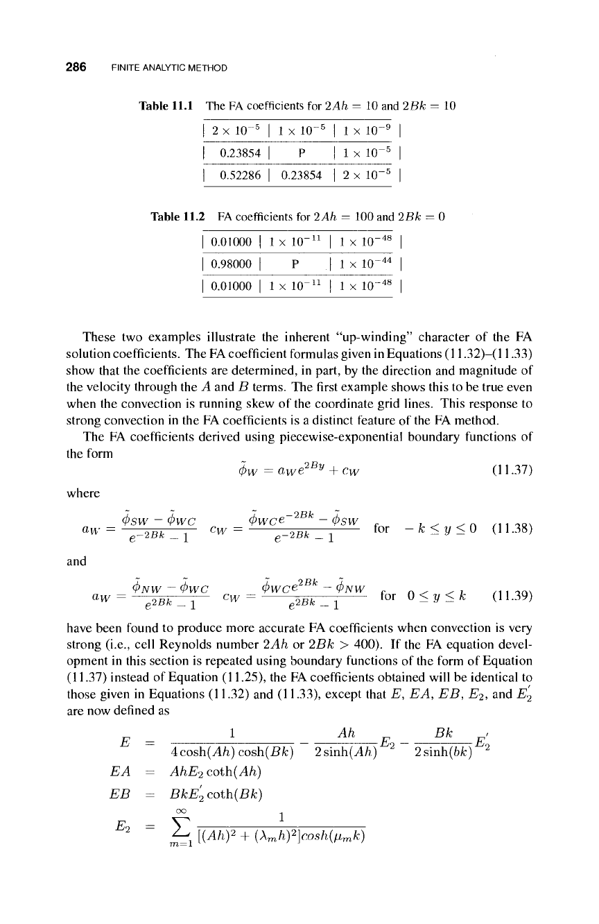
286 FINITE ANALYTIC METHOD

Table 11.1 The

coefficients for 2Ah = 10 and 2Bk =

| 2

10~

I 0.23854

| P |

10~

| 0.52286

0.23854

10~

Table 11.2

coefficients for 2Ah = 100 and 2Bk =

0.01000

10"

10~

0.98000

| P |

10~

0.01000

10"

These

two

examples illustrate

the

inherent "up-winding" character

the

solution coefficients. The FA coefficient formulas given in Equations (11.32)—(11.33)

show that the coefficients are determined, in part, by the direction and magnitude of

the velocity through the

and

terms. The first example shows this to be true even

when the convection

running skew

the coordinate grid lines. This response

strong convection in the FA coefficients is a distinct feature

the FA method.

The FA coefficients derived using piecewise-exponential boundary functions

the form

4>w

2By

+ c

(11.37)

where

4>sw-4>wc 4>wce~

2Bk

-4>sw

, . .

n nl

.n,

-2Bk_

°w =

-2Bk

_ !

for

<y<Q (H-38)

and

4>NW -

4>wc

4>wce

2Bk

- 4>NW ,

, . j

nnm

2Bk

_ !

^ =

2Bk

_ !

f0r

°<y<

(H·

)

have been found to produce more accurate FA coefficients when convection

very

strong (i.e., cell Reynolds number

2Ah or 2Bk >

400).

the FA equation devel-

opment in this section is repeated using boundary functions of the form of Equation

(11.37) instead of Equation (11.25), the FA coefficients obtained will be identical

those given

Equations (11.32) and (11.33), except that

E, EA, EB, E

and

are now defined as

1 Ah _ Bk .

Acosh(Ah)cosh(Bk) 2sinh(A/i)

2sinh(Wfe)

AhE

coth(Ah)

BkE

coth(Bk)

= Σ

; {(Ah)

]cosh(ß

2D TRANSPORT EQUATION 287

/ _ h

cosh(Bk) Ak · tcinh(Bk) - Bh · tanh(Aft)

~ k

cosh(Ah)

2AkBk · cosh(Ah)

with

yjA

+ B

+ X

and

_ (2m - 1)π

" 2h

The coefficients developed earlier in this section using exponential and linear

boundary functions, such as Equation (11.25) are more accurate than the piecewise-

exponential coefficients for the case of pure diffusion (i.e., no fluid flow). For

moderate cell Reynolds numbers, both formulations produce comparable coefficients.

Further discussion of this matter can be found in [5].

Other means for producing finite analytic solutions on small elements of the

computational domain have been used. Lowry and Li [21] use finite differences to

replace the Laplacian in the transport equation, and then find an analytic solution for

the first-order hyperbolic PDE that remains. Manohar and Stephenson [22] use real

and imaginary parts of powers of x + iy that form a complete basis for harmonic

functions. The local solution on a given element is approximated by a finite number

of terms whose coefficients are determined by matching element boundary values at

the element boundary nodes.

11.2.2 The Poisson Equation

Equation (11.20) reduces to the Poisson equation when φ = φ and R = 0.

The finite analytic solution of Equation (11.40) for node P(i,j) on the 2h x 2k FA

element is easily obtained from Equations (11.31) to (11.33) as

Ψ?= Σ

Cjuj+CpRfp

(11.41)

3=NE

where

C¿

and C

are the FA coefficients given in Equations (11.31) and (11.35) with

A = B = 0 (making them invariant because A = B = 0 always). For example, with

—

k, the FA coefficients are

CEC

— C

= C

= 0.205315

NW =

SE =

sw = 0.044685

and

= 0.294685ft

288 FINITE ANALYTIC METHOD

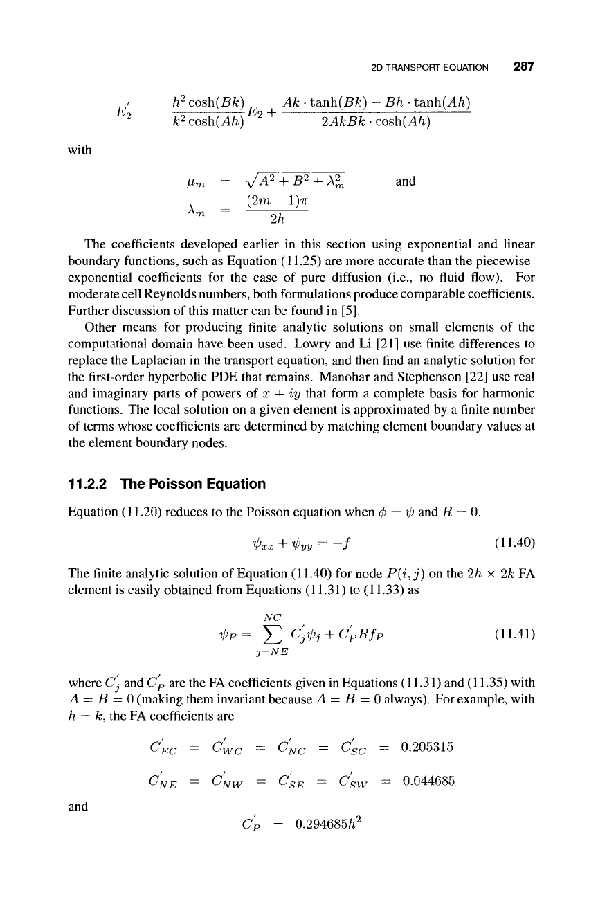
EXAMPLE 11.2 Poisson's Equation

The finite analytic method is used to solve the Poisson problem shown in BVP

(11.42).

A uniform grid spacing in x and y oí h

—

0.05 was used.

BVP

-V

u(x, y) = -2{y{l - y) + x(l - x)) (PDE)

u(x,2/)|an=0 (BC)

(11.42)

The true solution to this BVP is u(x, y) = (x

—

)(y

—

), and is used to

determine the accuracy of the FA solution. A plot of the FA solution is given

in Figure 11.7. The surface plot of the true solution is given as well. The FA

solution agrees remarkably well with the true solution.

0.2 0.4 0.6 0.8

0.8

0.2 0.4 0.6 0.8 1

(a) True solution. (b) FA solution.

Figure 11.7 True solution and

finite

analytic solution to the Poisson problem.

Laplace's equation results from Equation (11.40) when / = 0. The FA solution for

Laplace's equation, represented by Equation (11.41), compares very closely to the

fourth-order nine-point FD solution [19], which gives

}

and

0.2

0.05.

The next example is for the case of the 2D transport equation where both convection

and diffusion terms are included.

■ EXAMPLE 11.3 Convection-Diffusion

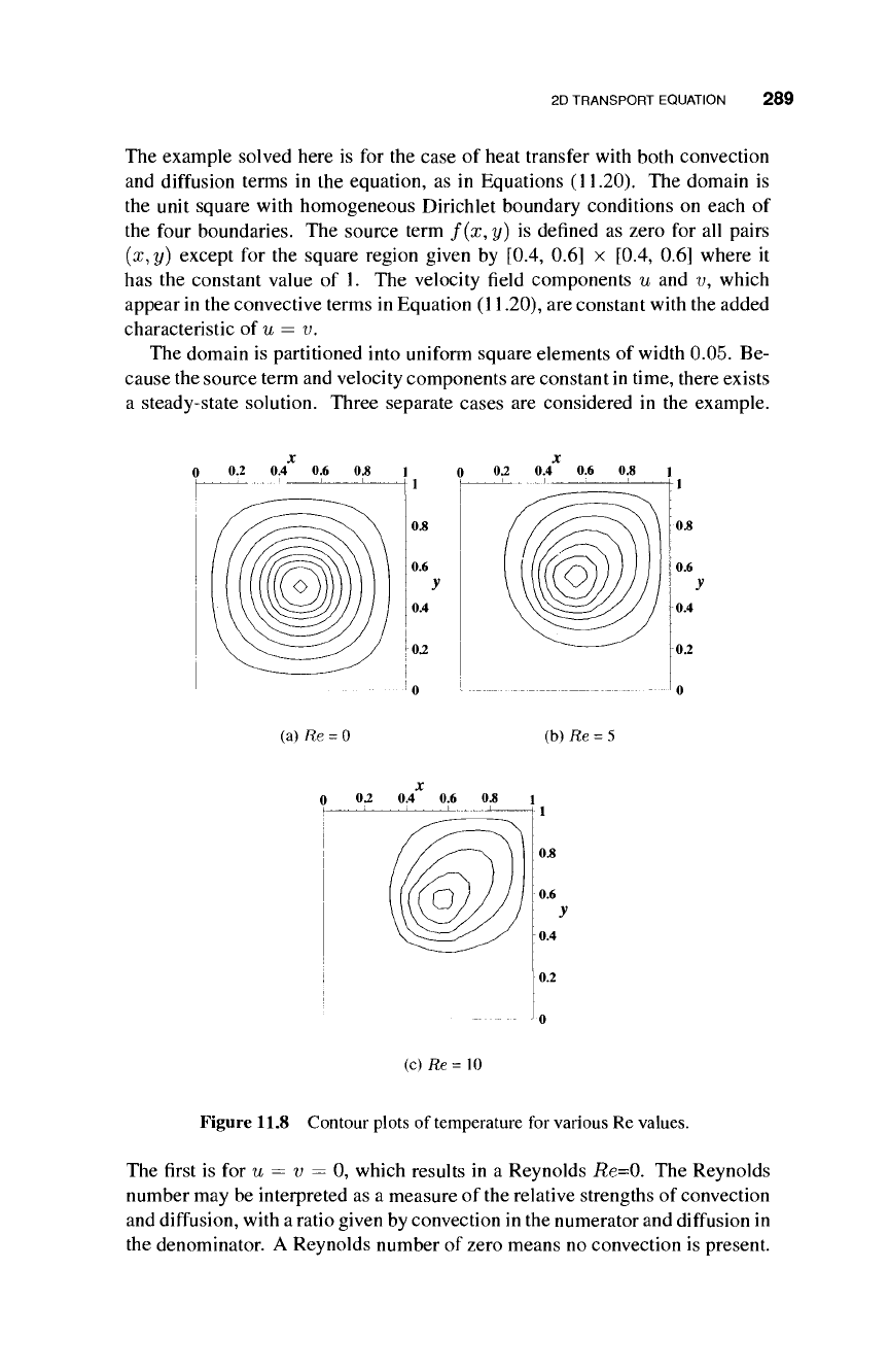
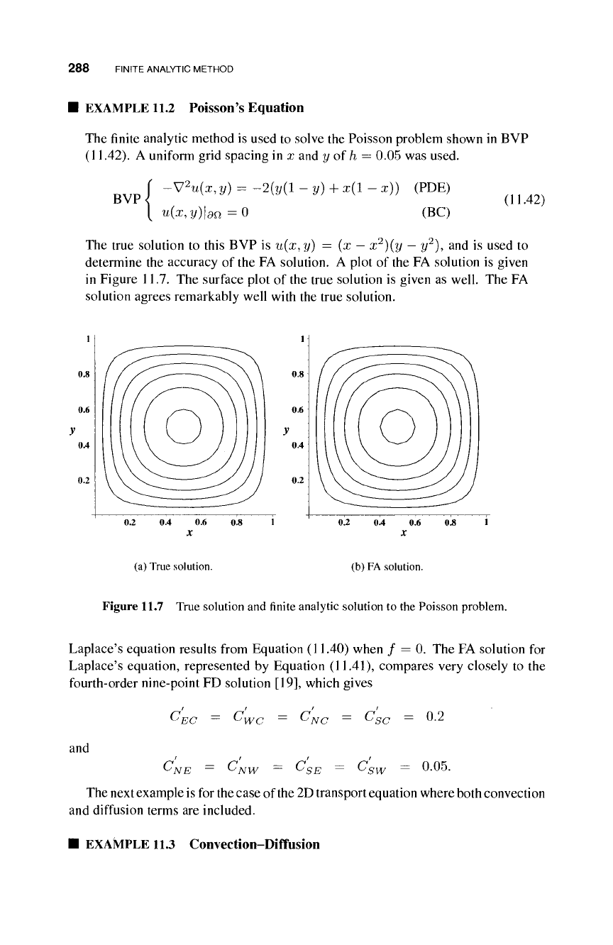
2D TRANSPORT EQUATION 289

The example solved here is for the case of heat transfer with both convection

and diffusion terms in the equation, as in Equations (11.20). The domain is

the unit square with homogeneous Dirichlet boundary conditions on each of

the four boundaries. The source term f(x,y) is defined as zero for all pairs

(x,

y) except for the square region given by [0.4, 0.6] x [0.4, 0.6] where it

has the constant value of 1. The velocity field components u and v, which

appear in the convective terms in Equation (11.20), are constant with the added

characteristic of u

—

The domain is partitioned into uniform square elements of width 0.05. Be-

cause the source term and velocity components are constant in time, there exists

a steady-state solution. Three separate cases are considered in the example.

x x

0 0.2 0.4 0.6 0.8 l 0 02 0.4 0.6 0.8 l

0.8

0.4

0.8

0.6

0.4

0.2

(a) Re

0 (b) Re

0 0.2 0.4 0.6 0.8 1

0.2

(c)Re= 10

Figure 11.8 Contour plots of temperature for various Re values.

The first is for u = v = 0, which results in a Reynolds Re=0. The Reynolds

number may be interpreted as a measure of the relative strengths of convection

and diffusion, with a ratio given by convection in the numerator and diffusion in

the denominator. A Reynolds number of zero means no convection is present.

290 FINITE ANALYTIC METHOD

The resulting contours, shown in Figure 11.8(a), are circular and centered on

the point (x, y) = (0.5,0.5) This case is considered as a means of comparing

results found for the nonzero convective cases.

The contour pattern for case two is shown in Figure 11.8(b). Here the

velocity field components are such that the resulting Reynolds number is "5."

Additionally, both u and v are positive, so there is a moderate "wind" blowing

from the southwest that skews the contour pattern to the northeast, as indicated

in Figure 11.8(b). The third case is similar to case two, but with a doubling of

the wind speed that gives a Re number of

"10."

Note how the contour pattern

shown in Figure 11.8(c) is skewed even further to the northeast than in the case

for Re = 05.

11.3 CONVERGENCE AND ACCURACY

This chapter concludes with a brief discussion of

the

convergence and accuracy of the

finite analytic method for the case of the 2D transport equation. The full details will

not be presented here. As with the other numerical methods introduced in this text,

the reader interested in the details is encouraged to consult the provided references.

The convergence of the finite analytic method for the case of the 2D transport

equations is established in the book by Chen et al. [10]. This is done by first showing

the method to be consistent, which is to say the norm of the difference between the

discrete version of the linear operator approximation to the nonlinear operator

F(</>)

R<t>

+ Ru(f)

Rv<t>y

- φ

χ - φ

and the operator F itself goes to zero as the uniform grid spacing h and temporal

spacing r approach zero. Next, the stability of the finite analytic method is estab-

lished by examining the resulting matrix of the linear operator approximation. This

matrix is based on the finite analytic coefficients found using the methods described

in Section 11.2. A numerical method is said to be stable if the resulting solution

varies, in a continuous way, on variations in the problem parameters, such as grid

spacing, operator coefficients, as well as boundary and initial conditions. The conver-

gence of the finite analytic solution to the true solution of the original IBVP follows

immediately from the consistency and stability of the method [20].

The order of convergence is established in the work by Peterson [29]. Two ap-

proached were used to study the spatial discretization error. In the first, the boundary

conditions were assumed to be exact for any arbitrary finite analytic element. If so,

the only source of error for the objective value of φ at the center node would be that

due to truncation error in the partial sum approximation to the Fourier series solution.

The truncation error is independent of the grid spacing, so the finite analytic solution

is "exact" relative to the grid spacing. A Taylor series approximation to the actual

boundary condition for an arbitrary finite analytic element is considered in the second

approach. Here, the finite analytic solution is shown to be a third-order methods in

the uniform grid spacing. Because the finite analytic method uses a forward finite

EXERCISES

291

difference

time

approximate

the

temporal derivative,

the

resulting convergence

is first order

in r.

Earlier work

Vanka

[31]

explored, experimentally,

the

accuracy

of the

finite

analytic method through calculations

multidimensional scalar transport.

The

velocity field

was

assumed

to be

uniform

and

directed

in a

skewed fashion

to the

grid lines. Results showed

the FA

method

to be

superior

results found

finite

difference methods.

The FA

method

did

show appreciable error

regions

steep

gradients, large grid Peclet numbers,

and

cases

skewed flow streamlines.

The

difficulty with steep gradients

usually overcome with increases nodal density

the direction

the gradient (perpendicular

physical boundaries, e.g.). Instead

using uniform grid with higher density throughout

the

domain,

it is

more efficient

use non-uniform spacing. Consequently,

the

finite analytic coefficient formulas

are

derived

for

such nonuniform spacing.

The

reader

referred

Chen

et al. [6] for

details

on the

method

for

nonuniform grids.

EXERCISES

11.1 Provide

the

details

transforming Equation (11.1) into

its

nondimensional

form, given

Equation (11.2), through

the use of

reference quantities

T, L, and Φ

for time, length,

and the

scalar quantity

φ,

respectively.

11.2 Using

the

change

variable

. (2Ax + Bt)F

= Φ

~ 4Α1 + Β*

show that Equation (11.4) results from Equation (11.3).

11.3 Use the hybrid FA method present in Section 11.1.3

solve Berger's equation

as presented

Section 11.1.

Use a

uniform spatial grid with

h =

0.01

and a

step size

r =

0.1.

Compare your results with those presented

Section 11.1.

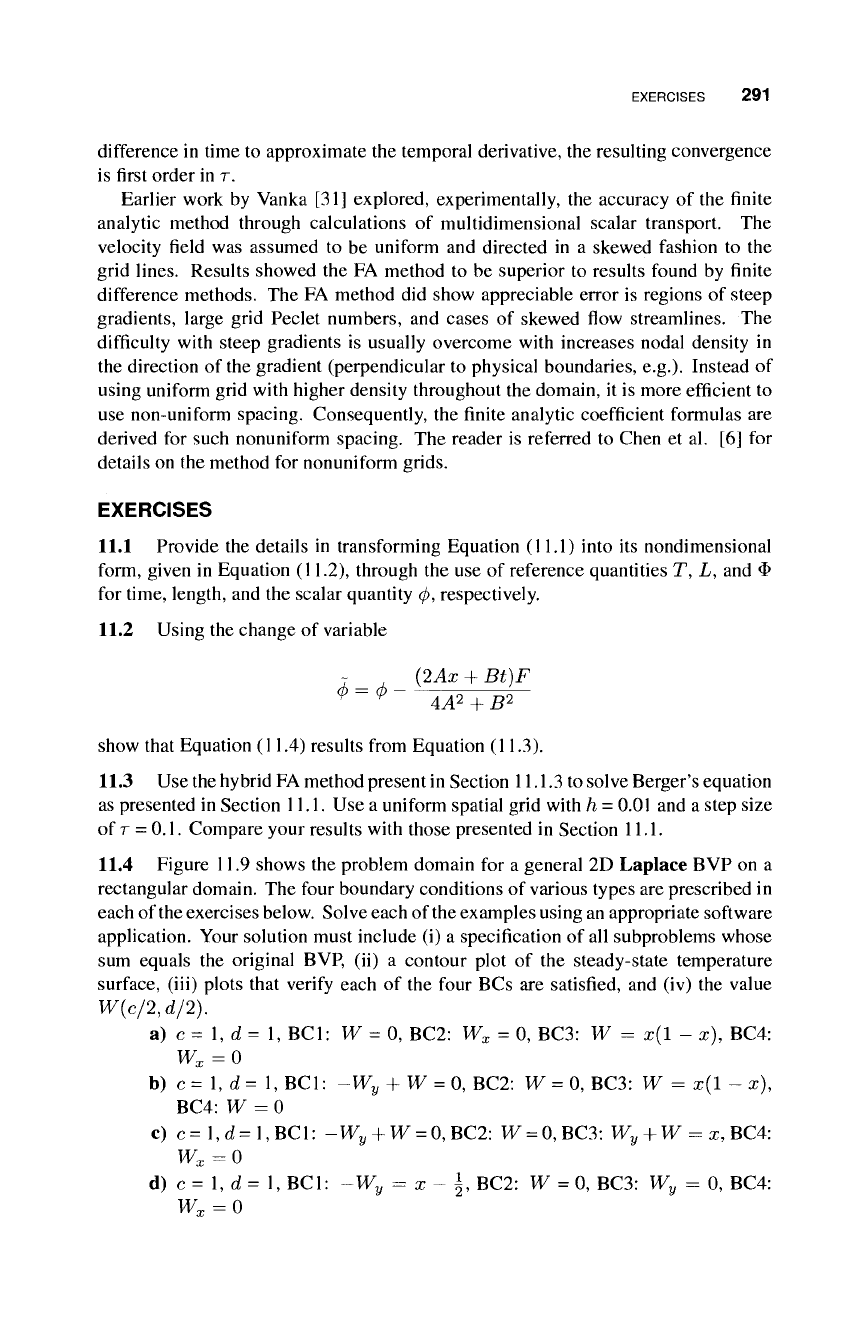
11.4 Figure

11.9

shows

the

problem domain

for a

general

Laplace

BVP on a

rectangular domain.

The

four boundary conditions

various types are prescribed

each of the exercises below. Solve each of the examples using an appropriate software

application. Your solution must include

(i) a

specification

all subproblems whose

sum equals

the

original

BVP, (ii) a

contour plot

of the

steady-state temperature

surface,

(iii)

plots that verify each

of the

four

BCs are

satisfied,

and (iv) the

value

W{c/2,d/2).

c = 1, d

BC1:

W = 0,

BC2:

BC3:

W = x(l - x), BC4:

1, d

BC1:

-W

+ W

BC2:

BC3:

W = x(l - x),

BC4:

W = 0

c) c=l,d=l,BCl:

-W

+ W

0,BC2:

W =

0,BC3:

+ W = x,

BC4:

1, d

BC1:

-W

= x - \,

BC2:

BC3:

= 0, BC4: