Bhushan B. Handbook of Micro/Nano Tribology, Second Edition

Подождите немного. Документ загружается.

2.9.3 Stand-Alone Setup

The disadvantage of the classical AFM setup is that the sample size is limited, both by the acceleration

power of the scanning system and by the allowable size. Many samples are of extended size and often it

is not desirable to cut them into small pieces. Therefore, a design where the force sensor is scanned past

the sample is desirable. A ﬁrst implementation (Bryant et al., 1988) used tunneling from the force sensor

to the tip to detect the deﬂection of the cantilever. In environments such as the ambient where adsorbate

layers cover both the cantilever and the tunneling tip, there might be problems adjusting the force (Marti

et al., 1988; Meyer and Amer, 1988; Alexander et al., 1989) The adsorbate layer between the tip and the

cantilever can stiffen the cantilever and induce unwanted large forces.

By using the interaction of light backscattered by a cantilever into a laser diode (Sarid et al., 1988;

Sarid et al., 1989, 1990), it was possible to build a compact AFM, where the cantilever was scanned. This

system, however, was not able to measure lateral forces.

Realizing that the divergence angle of a light beam reﬂected from a cantilever is given either by the

focal diameter or by the width of the cantilever (whichever is smaller) (Colchero, 1993), it was found

that by using a rather broad laser beam with a focal diameter of 50 µm one could safely displace the

cantilever for more than 10 µm laterally without any unwanted cross talk, provided the light was incident

perpendicularly to the cantilever (Hipp et al., 1992) (see Figure 2.27). This can be achieved with the setup

shown in Figure 2.28. A laser diode serves as a light source, and the linearly polarized light passes through

a polarizing beam splitter and a quarter wave plate. The laser is focused onto the cantilever. Since the

light is incident perpendicularly on the cantilever, its polarization state will not change. For all other

angles of incidence, the s- and p-polarized light will have different reﬂectivities. The cantilever now

deﬂects the light according to the force acting on it. The deﬂection angles are of the order of microradians

and, hence, negligible. The returning circularly polarized light is converted to linear polarized light by

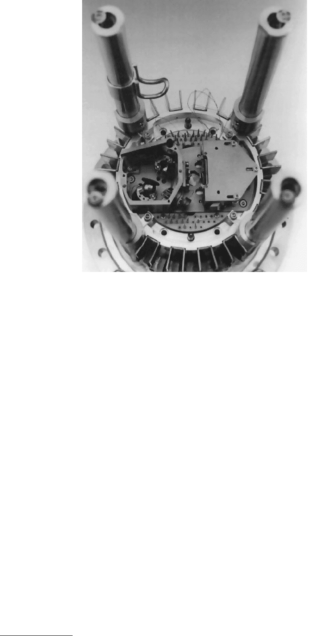
FIGURE 2.25 View of a commercial AFM for ultrahigh vacuum operation. (Courtesy of Omicron. Used with

permission.)

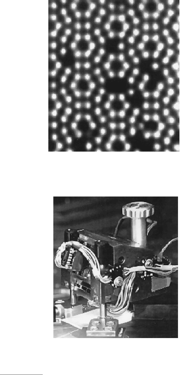
FIGURE 2.26 Silicon (111) surface measured by noncontact atomic force microscopy. (Courtesy of Omicron. Used

with permission.) The color scale corresponds to the frequency shift in the oscillation of the cantilever. It is a measure

of the interaction strength.

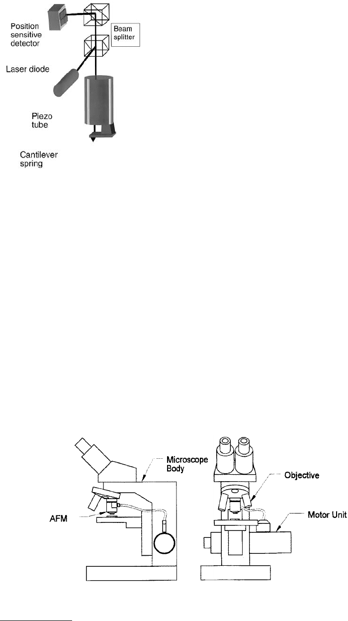
FIGURE 2.27 An implementation of the stand-alone principle discussed above. (From Hipp, M. et al., 1992,

Ultramicroscopy, 42–44, 1498–1503. With permission.)

the quarter wave plate. The linear polarization state is orthogonal to the incident one. Therefore, the

polarizing beam splitter cube now keeps the returning light away from the laser and directs it to the

quadrant diode. The main limitation of this setup is the limited scanning range, due to the focal diameter

of the laser beam.

As was discussed in the section on scanning systems, there are powerful long-range scanners available

nowadays using piezostacks and solid-state joints. These scanners can also serve as a mount for the optical

beam deﬂection system. Since the entire optics are scanned, the problem of the cantilever moving out

of the focus of the laser beam is absent. The scanning range is only limited by the available stroke of the

translation table. Some commercial instruments are based on this principle.

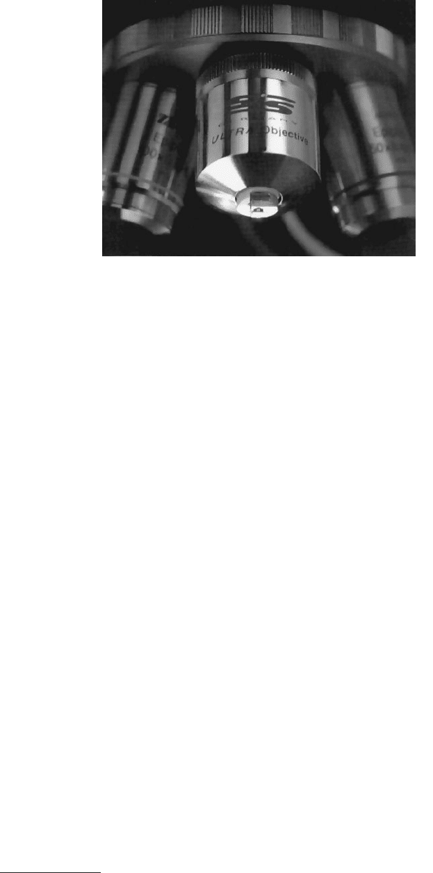
An exciting new development is the integration of an AFM into the lens holder of a classical microscope,

as shown in Figure 2.29. A detailed view of this principle is shown in Figure 2.30. This microscope has

a scan range of larger than 30 µm, combined with a resolution of better than 1 nm. Only a clever

arrangement of components and extreme miniaturization made it possible to design it. The objective

contains everything, from scanners to the approach unit.

2.9.4 Data Acquisition

The interaction between the tip and the sample is usually of very short range. The range of the interaction

is inversely proportional to the potentially achievable resolution.The tunneling current in the STM, in

particular, changes approximately by an order of magnitude for a distance change of the

separation of

FIGURE 2.28 Optical path in a stand-alone AFM. The incident light

impinges perpendicularly onto the cantilever. A quarter wave plate

serves as a separator for the incoming and the outgoing light.

FIGURE 2.29 A sketch of the mounting principle of the SIS stand-alone instrument. (Courtesy of SIS. With

permission.)

100 pm. However, many surfaces have surface features with height differences that are much larger than

the range of the control interaction. Therefore, the probe height above the sample has to be adjusted to

avoid uncontrolled contact with the sample or the loss of information.

The height of the probe above the sample is controlled by a feedback loop (Park and Quate, 1987;

Marti et al., 1988; DiLella et al., 1989; Piner and Reifenberger, 1989; Troyanovskii, 1989; Grafström et al.,

1990; Jeon and Willis, 1991; Schummers et al., 1991). A schematic sketch of such a feedback loop was

shown in Figure 2.20. The probe tip or, alternatively, the sample is connected to a converter which outputs

a voltage proportional to the interaction between the tip and the sample. The output of the converter is

low-pass ﬁltered and fed into a linearizing network, whose output is compared with a preset voltage. The

difference voltage or error voltage is fed into a feedback control ampliﬁer. The simplest of those ampliﬁers

consists of an integrator. To speed up the response of the instrument, proportional and differential gain

can be added (DiStefano et al., 1976). The resulting signal controls the high-voltage ampliﬁers for the

z-piezotranslator. The feedback systems has stringent requirements: in an STM it is not tolerable if the

overshoot at a step is larger than 100 pm. Set into relation with a typical z-range of 1 µm the precision

must be 0.01%. Likewise, the noise level must be of even better quality. High gain minimizes the error

margin of the control interaction and forces the tip to follow the contours of constant-interaction signal

magnitude as well as possible. This mode of operation is known as the “constant-interaction” mode. The

information on the surface topography can be found in the control signal for the z-piezo. The “constant-

height” mode is used for ﬂat samples. The probe tip is scanned across the sample without feedback

control. The variations of the interaction signal reﬂect the topography. Linear interactions such as that

in contact-mode AFM are easy to translate into true heights of the sample surface.

Signal generators produce the drive voltages for the x- and y-scan piezos. Usually the fast scan direction

is labeled by x. Its scanning frequency might be as high as 1000 Hz. The y-scan frequency is lower by the

number of lines in the image.

The feedback control and scan generation system can be implemented with analog electronics or with

digital signal processors. While digital feedback control offers greater ﬂexibility in the choice of the

frequency response, allows adaptive controls, and is easy to reconﬁgure (Aguilar et al., 1986, 1987; Becker,

1987; Brown and Cline, 1990; Baselt et al., 1993), analog feedback circuits might be better suited for

ultralow noise operation.

The basic feedback loops can be expanded to allow a wide variety of imaging modes. Often the feedback

loop can be interrupted and the position of the probe tip or the control voltages or signal are varied.

The response of the probe signal is sampled. This mode of imaging is called “spectroscopic imaging”

FIGURE 2.30 The stand-alone microscope Ultra-Objective™ from SIS. (Courtesy of SIS. With permission.)

(Baratoff et al., 1986; Hamers et al., 1986; Stroscio et al., 1986; Bell et al., 1990; van Kempen, 1990;

Schummers et al., 1991).

2.9.4.1 Sampling Theorem Applied to AFM

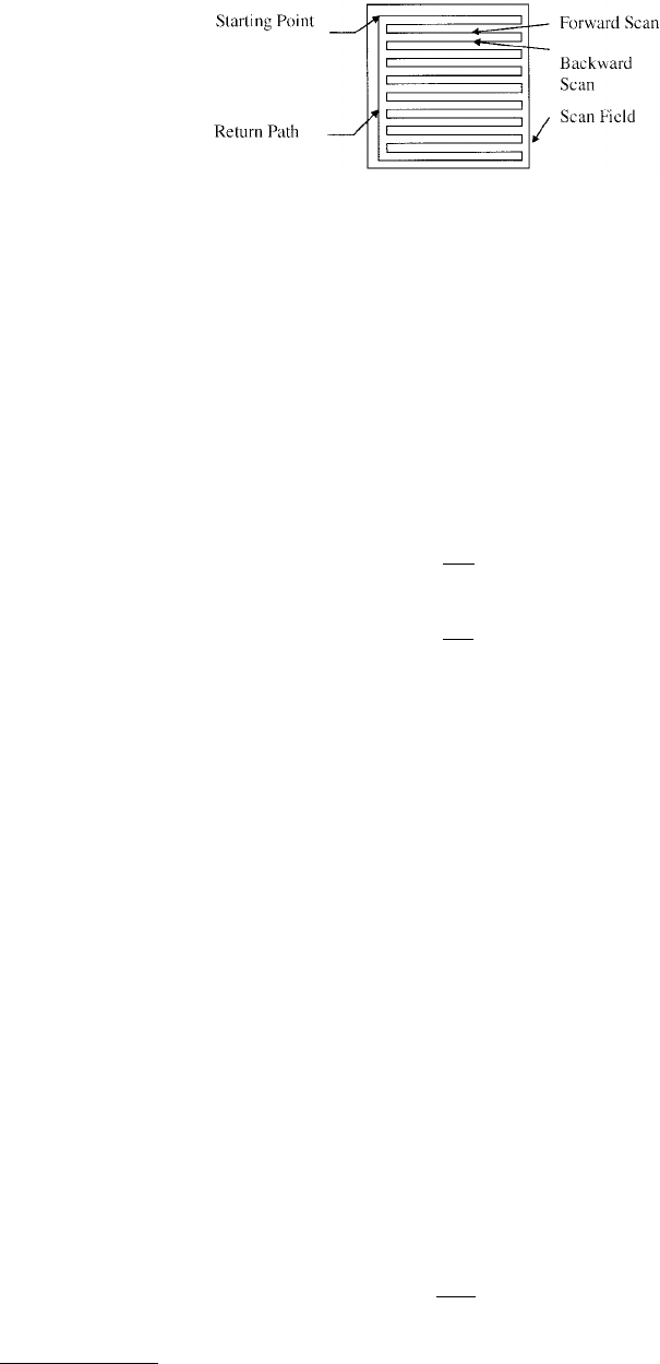
AFMs acquire the data in a raster scan fashion. This means that the surface is probed in lines, one adjacent

to the other. In each line there are only a limited number of points. Figure 2.31 shows a typical scan

pattern. There are variations to this pattern. The backward scan can be on the same line as the forward

scan. The sample can be scanned backward from the bottom to return to the starting point.

The scanning pattern is characterized by the number of points along the line N

and the number of

lines N

. If the size of the scanning pattern is x

by y

, then one can calculate the distance between two

points or two lines. We obtain

(2.96)

Assume that the sample has features with a characteristic size of x

and y

. These characteristic sizes can

only be resolved if the following inequalities hold:

(2.97)

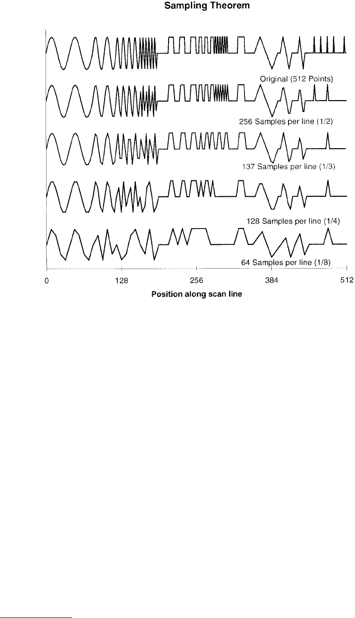
Equation 2.97 is a fundamental limitation of sampling data (Yaroslavski, 1985). It is intuitively clear that,

if one wants to measure a sine, one has to sample at least two points per period. If this effect is not

observed, one can get data at the wrong positions. Figure 2.32 shows a simulation of this effect. It is

obvious that, for instance, the sine with period 5 is not sampled correctly at one quarter of the sampling

points. The dangerous thing is that due to aliasing a wrong period is appearing. A similar effect can be

seen for the square waves with a period 4. Even at one third the sampling rate, one misses the true

periodicity, since the sampling theorem is violated. The single point spikes above 450 are imaged or not,

depending on the sampling rate.

The conclusion from this experiment is that if one wants to image something with a characteristic

distance of, for example, 1 nm, then one needs at least 200, better 600, data points if the ﬁeld of view is

100 nm on the side. Otherwise, one is bound to have aliasing effects and, consequently, moiré patterns

and a loss of information.

Since a sampling spacing in real space is translated to a frequency by the scanning speed, one can also

apply the sampling theorem to frequency.

(2.98)

FIGURE 2.31 Scan pattern in an AFM.

∆

Equation 2.98 shows this effect for the fast scanning direction. In frequency the sampling theorem means

that the digitizing rate needs to be at least twice as high as the highest frequency in the signal. An example

demonstrates this. If one wants to measure something with a 1-nm periodicity at a scanning speed of

1 µm/s at least 2000 samples per second are needed, better yet 12,000 samples per second. In the

time/frequency domain it is easy to prevent aliasing. Just use a low-pass ﬁlter with the maximum allowable

frequency (the Nyquist frequency) in front of the analog-to-digital converter. It prevents aliasing. If the

sampling theorem is violated, then nothing will be seen.

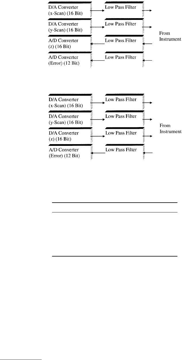
2.9.5 Typical Setups

The analysis of the sampling theorem suggests that a typical setup for the analog-to-digital conversion

should look like Figure 2.33 or Figure 2.34. The difference between the two ﬁgures lies in the fact that

for an analog feedback circuit one has to digitize the topographical signal, which is at the output of the

feedback controller, whereas in a digital feedback circuit the computer calculates the z-signal from the

error signal. In both cases, one must match the cutoff frequency of the low-pass ﬁlters to the conversion

rate of the digital-to-analog (D/A) or analog-to-digital (A/D) converters.

The precision of the converters limits the resolution; 16 bits are equal to one part in 65,536. By

observing the sampling theorem, this means that the smallest object must be 32,768 times smaller than

FIGURE 2.32 Effect of the sampling theorem. The successive lines from the top to the bottom are the original and

sampled data. The original contains the following objects (from the left side): sine with period 40 (from 0 to 80),

sine with period 20 (from 80 to 120), sine with period 10 (from 120 to 160), sine with period 5 (from 160 to 190),

a square wave with period 18 (190 to 256), a square wave with period 10 (256 to 286), a square wave with period 4

(286 to 310), a single square pulse of width 12 between 310 and 356, a triangle of period 40 between 356 and 396,

a triangle of period 20 between 400 and 420, a triangle of period 12 between 430 and 442, and, ﬁnally, delta pulses

(1 wide) at 458, 469, 480, 491, and 509.

the scanning range. Table 2.3 shows a compilation of the resolution as a function of the most common

maximal scanning ranges and some D/A (or A/D) converter resolutions. Since the 16-bit converters are

very common (because of the CD–audio market), most instruments use this resolution. A 100-µm scanner

is capable of resolving a little bit more than 1 nm.

2.9.6 Data Representation

The visualization and interpretation of images from SPMs is intimately connected to the processing of

these images.

An ideal scanning probe microscope is a noise-free device that images a sample with perfect tips of

known shape and has perfect linear scanning piezos. In reality, AFMs are not that ideal. The scanning

device in AFMs is affected by distortions. To do quantitative measurements, such as determining the unit

cell size, these distortions have to be measured on test substances and have to be corrected for. The

FIGURE 2.33 Typical setup of a data acquisition system with an analog feedback circuit.

FIGURE 2.34 Typical setup of a data acquisition system with a digital feedback system.

TABLE 2.3 Sampling Resolution (in nanometers) as a

Function of the Scan Range and the Converter Resolution

8 Bit 12 Bit 16 Bit 18 Bit 20 Bit

1 nm 0.008 4.9E-04 3.1E-05 7.6E-06 1.9E-06

10 nm 0.078 4.9E-03 3.1E-04 7.6E-05 1.9E-05

100 nm 0.78 0.05 0.003 7.63E-04 1.91E-04

1 µm 7.81 0.49 0.031 0.008 0.002

10 µm 78.13 4.88 0.31 0.08 0.02

100 µm 781.25 48.83 3.05 0.76 0.19

250 µm 1953.13 122.07 7.63 1.91 0.48

distortions are both linear and nonlinear. Linear distortions mainly result from imperfections in the

machining of the piezotranslators causing cross talk from the z-piezo to the x- and y-piezos, and vice

versa. Among the linear distortions, there are two kinds which are very important: ﬁrst, scanning piezos

invariably have different sensitivities along the different scan axes due to the variation of the piezo material

and uneven sizes of the electrode areas. Second, the same reasons might cause the scanning axis to not

be orthogonal. Furthermore, the plane in which the piezoscanner moves for constant z is hardly ever

coincident with the sample plane. Hence, a linear ramp is added to the sample data. This ramp is especially

bothersome when the height z is displayed as an intensity map, also called a top-view display.

The nonlinear distortions are harder to deal with. They can affect AFMs for a variety of reasons. First,

piezoelectric ceramics do have a hysteresis loop, much like ferromagnetic materials. The deviations of

piezoceramic materials from linearity increase with increasing amplitude of the driving voltage. The

mechanical position for one voltage depends on the voltages applied to the piezo before. Hence, to get

the best position accuracy, one should always approach a point on the sample from the same direction.

Another type of nonlinear distortion of the images occurs when the scan frequency approaches the upper

frequency limit of the x- and y-drive ampliﬁers or the upper frequency limit of the feedback loop

(z-component). This distortion, due to the feedback loop, can only be minimized by reducing the scan

frequency. On the other hand, there is a simple way to reduce distortions due to the x- and y-piezo drive

ampliﬁers. To keep the system as simple as possible, one normally uses a triangular waveform for driving

the scanning piezos. However, triangular waves contain frequency components at multiples of the scan

frequency. If the cutoff frequency of the x- and y-drive electronics or of the feedback loop is too close

to the scanning frequency (two to three times the scanning frequency), the triangular drive voltage is

rounded off at the turning points. This rounding error causes, ﬁrst, a distortion of the scan linearity and,

second, through phase lags, the projection of part of the backward scan onto the forward scan. This type

of distortion can be minimized by carefully selecting the scanning frequency and by using driving voltages

for the x- and y-piezos with waveforms like trapezoidal waves, which are closer to a sine wave. The values

measured for x, y, or z are affected by noise. The origin of this noise can be either electronic, some

disturbances, or a property of the sample surface due to adsorbates. In addition to this incoherent noise,

interference with mains and other equipment nearby might be present. Depending on the type of noise,

one can ﬁlter it in the real space or in Fourier space. The most important part of image processing is to

visualize the measured data. Typical AFM data sets can consist of many thousands to over a million

points per plane. There may be more than one image plane present. The AFM data represents a topo-

graphy in various data spaces.

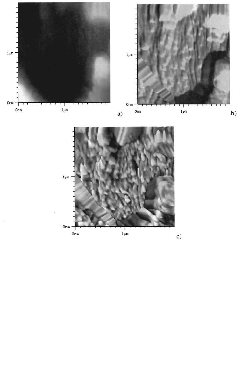
We use data from a combined measurement of topography, stiffness, and adhesion to outline the

different points of data processing. Figure 2.35a shows the topography, Figure 2.35b the local stiffness

image, and Figure 2.35c the adhesion image acquired simultaneously, as described in (Marti et al., 1997).

The same data can be rendered as a series of consecutive cross sections. Figure 2.36 is an example. Line

renderings can be excellent to judge the general form of the topography, independent of color settings.

The original data set contains 256 lines with 256 points each. Since it is not possible to draw 256 distinct

lines, the data in Figure 2.36 show every sixth line. Along the lines, all the points are drawn.

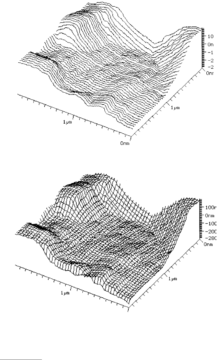
Similarly, the data can also be rendered in a wire mesh fashion (Figure 2.37). Again, a line is drawn

at every sixth point both in the horizontal and vertical direction. It is especially suitable for monochrome

display systems with only two colors. The number of scan lines that can be displayed is usually well below

100 and the display resolution along the fast scanning axis x is much better than along y.

If the computer display is capable of displaying at least 64 shades of gray, then top-view images can

be created (Figure 2.38). In these images, the position on the screen corresponds to the position on the

sample and the height is coded as a shade of gray. Usually, the convention is that the brighter a point,

the higher it is. The number of points that can be displayed is only limited by the number of pixels

available. This view of the data is excellent for measuring distances between surface features. Periodic

structures show up particularly well on such a top view. The human eye is not capable of distinguishing

more than 64 shades of gray. If the average z-height of the tip varies from one side of the image to the

other, then the interesting features usually have too little contrast. Hence, contrast equalization is needed.

For data being affected by a large background slope, it is often still possible to detect some features in

the line scan view. Some researchers prefer a simultaneous display of both line scan images and top-view

images to get the most information in the shortest time. Top views use much less calculation time than

line scan images. Hence, computerized fast data acquisition systems usually display the data as a top view

ﬁrst.

Figure 2.35 shows in a detailed way what the topography of the sample is. However, the ﬁne details

in the low-lying parts are obscured. There are simply not enough shades which the eye can distinguish.

The display can be enhanced by adding some illumination to it. In illuminated data sets one depicts the

cosine of the angle between the surface normal and some predeﬁned direction, the illumination direction.

This technique is a powerful tool to enhance the appearance of a data set, but it can be abused! Changing

the direction of the light source, as shown in Figure 2.39, can obscure some undesired features.

The effect of the illumination is similar to displaying the magnitude of the gradient of the sample

surface along the direction to the light source. Features perpendicular to the illumination cannot be seen.

FIGURE 2.35 A rubber sample: (a) shows the topography, (b) the local stiffness, and (c) the adhesion.

Multiple light sources or extended light sources diminish this effect, but the illumination is much more

complicated to calculate. If not shown in conjunction with some other display method, one is not able

to judge the validity of such an image.

FIGURE 2.36 A line rendering of the topography (Figures 2.35).

FIGURE 2.37 A wire mesh rendering of the topography of a rubber sample (Figure 2.35).