Bhushan B. Handbook of Micro/Nano Tribology, Second Edition

Подождите немного. Документ загружается.

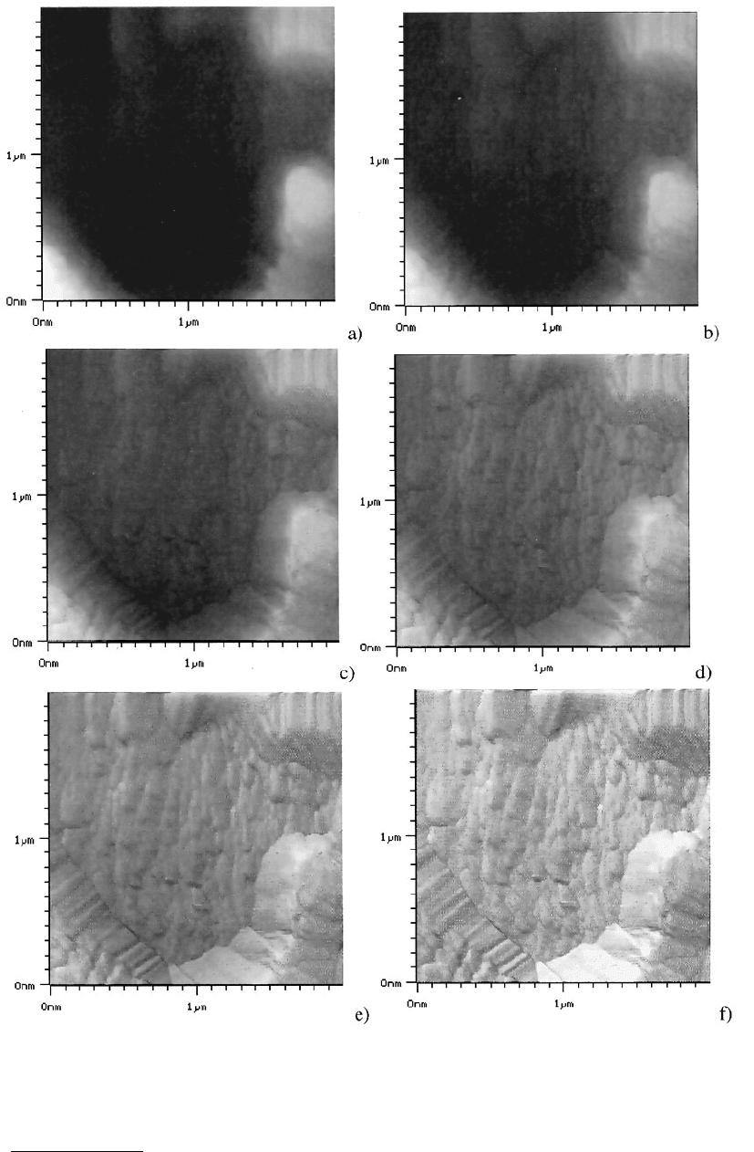
FIGURE 2.38 Variation of the light added to a topography. (a) is the topography without any light (the same as

Figure 2.35). (c) is the same data, but rendered with a light source from the right at 50° elevation. (b) has 20% light

added, (c) 40%, (d) 60%, (e) 80%, and (f) 100%.

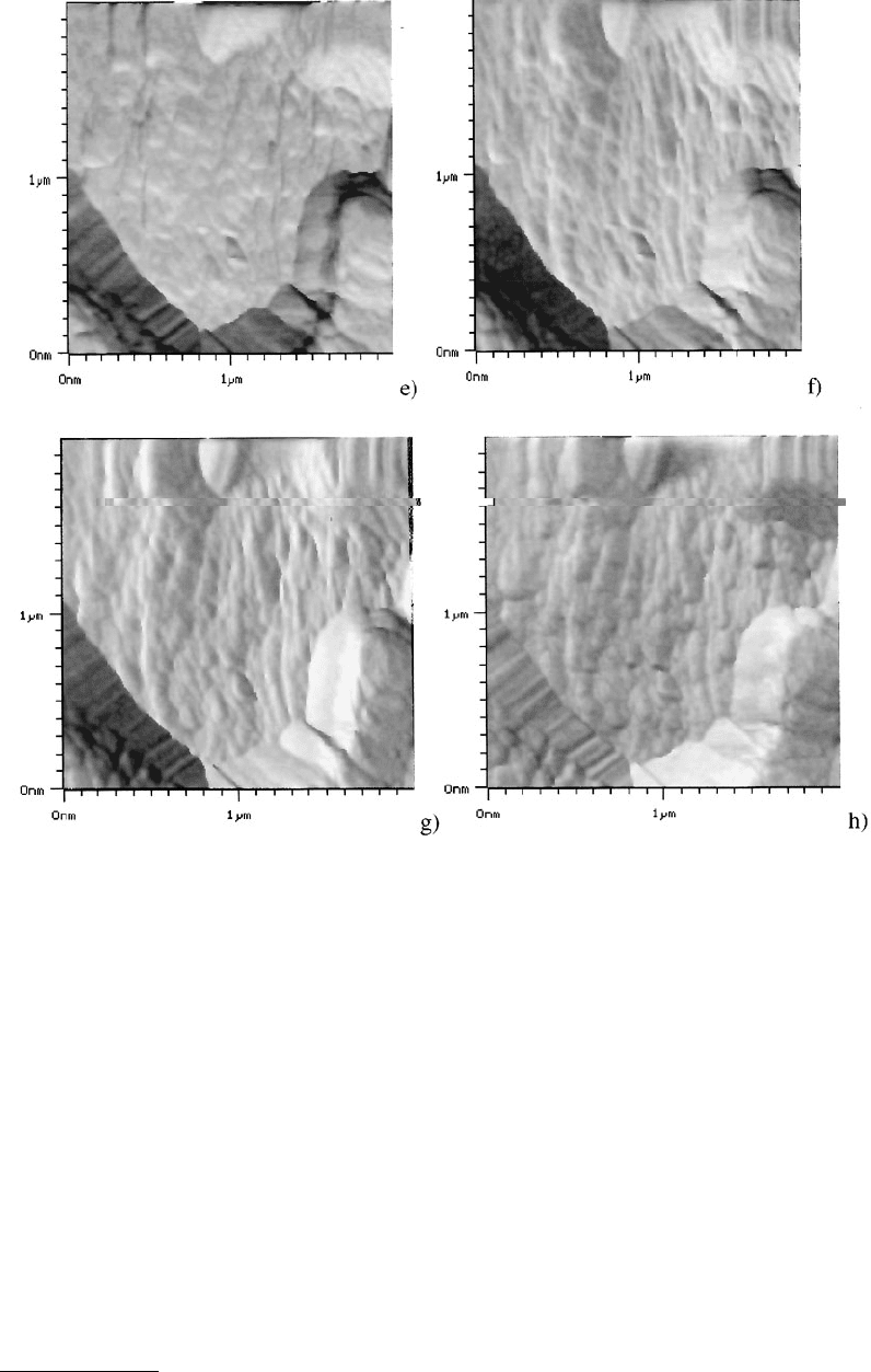
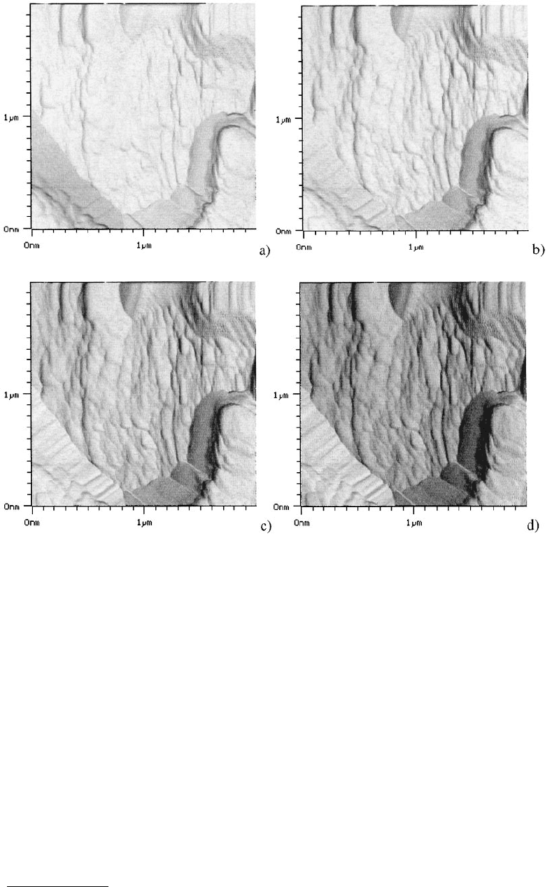
Figure 2.40 shows the inﬂuence of the elevation angle on the displayed image. It is clear that an

illumination from about 30° to 60° is optimal. One can combine top views or illuminated top views and

wire mesh scan displays to form solid surface models of the sample surface. Such images are usually only

generated in the ﬁnal processing stage before publication, because they need quite a lot of computing time.

Continuous shading techniques sometimes make it difﬁcult to analyze the topography. By using

discontinuous color tables, one can create something similar to contour maps. An example is shown in

Figure 2.41.

Figure 2.42 shows a combination of the top view display and the wire mesh display, a three-dimensional

model where the height is coded as a shade of gray. As with the top view (Figure 2.35), one can vary the

amount of illumination added to the data. Figures 2.42 through 2.47 show the inﬂuence of the amount

of illumination in the display.

Data consisting of more than one channel can be packed into one three-dimensional image. One

channel, usually the topography, is used to model the height, whereas the second channel is used to

produce the shades. Figure 2.48 shows the topography shaded with the stiffness. Figure 2.49 shows the

same data, but colored with the topography.

FIGURE 2.39(a–d)

Additional information can be packed into an image by using color. Assume that an image has two

planes of data. We can display the ﬁrst plane with shades of green and the second one with shades of red

on top of each other. Where the magnitude of both planes is high, one gets an orange color; where both

are low, one gets black. But if the magnitude of one plane is larger than that of the other plane on one

pixel, one gets red or green colors. This way, one can display the registry of two different quantities in

the same image.

2.9.7 The Two-Dimensional Histogram Method

To analyze quantitatively friction microscopy data, one would like to calculate local friction coefﬁcients.

Normally, one operates a friction microscope in the constant-force mode, recording the topography z(x,y)

and the lateral force F

(x,y). If the normal force F

is kept constant, one can get a local friction coefﬁcient

γ(x,y) = F

(x,y)/F

. γ(x,y) is well deﬁned, if the normal force F

is truly constant, if the calibrations of

both forces are known, and, most crucially, if the zero points of the force scales are known and stable.

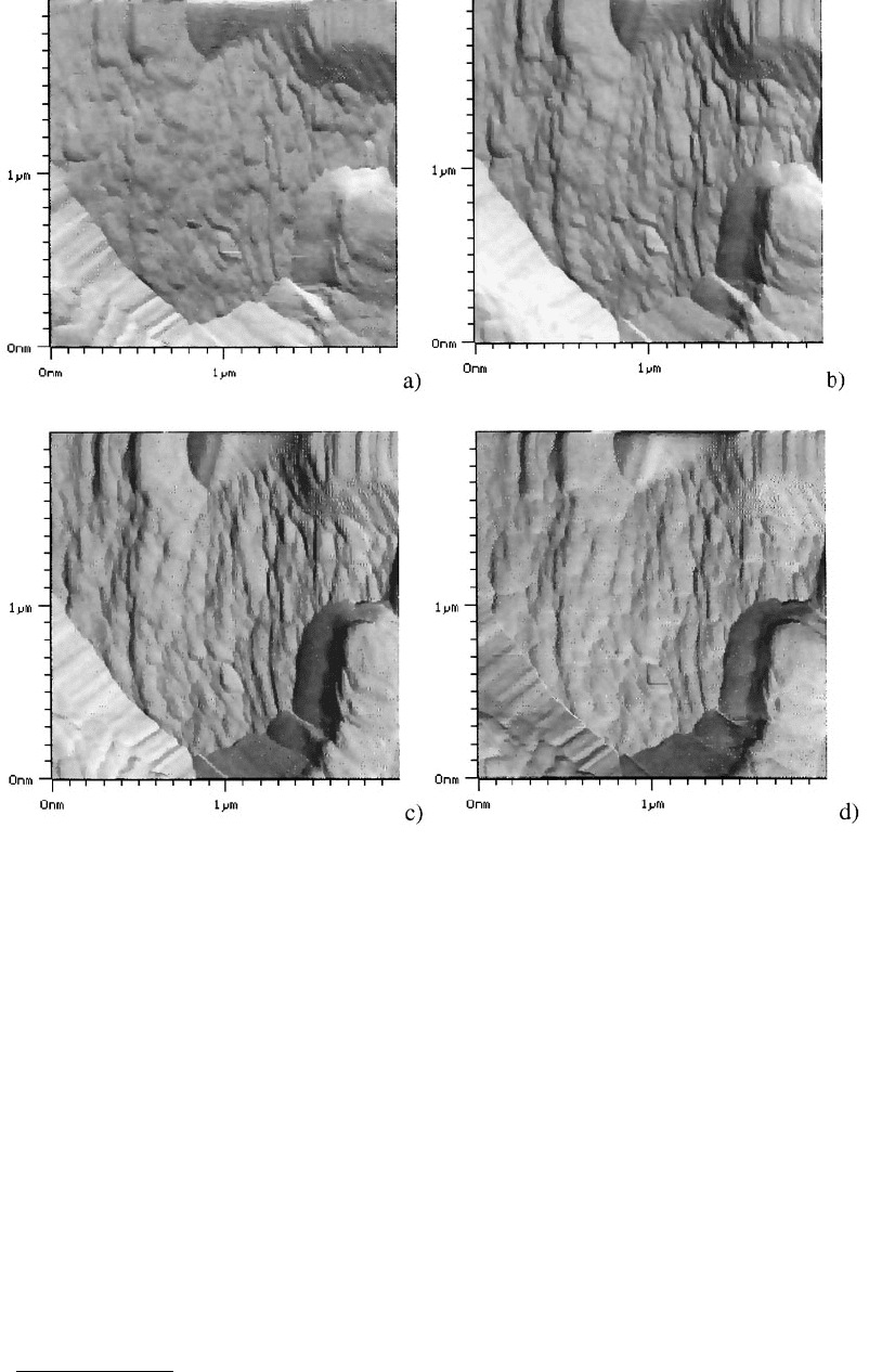
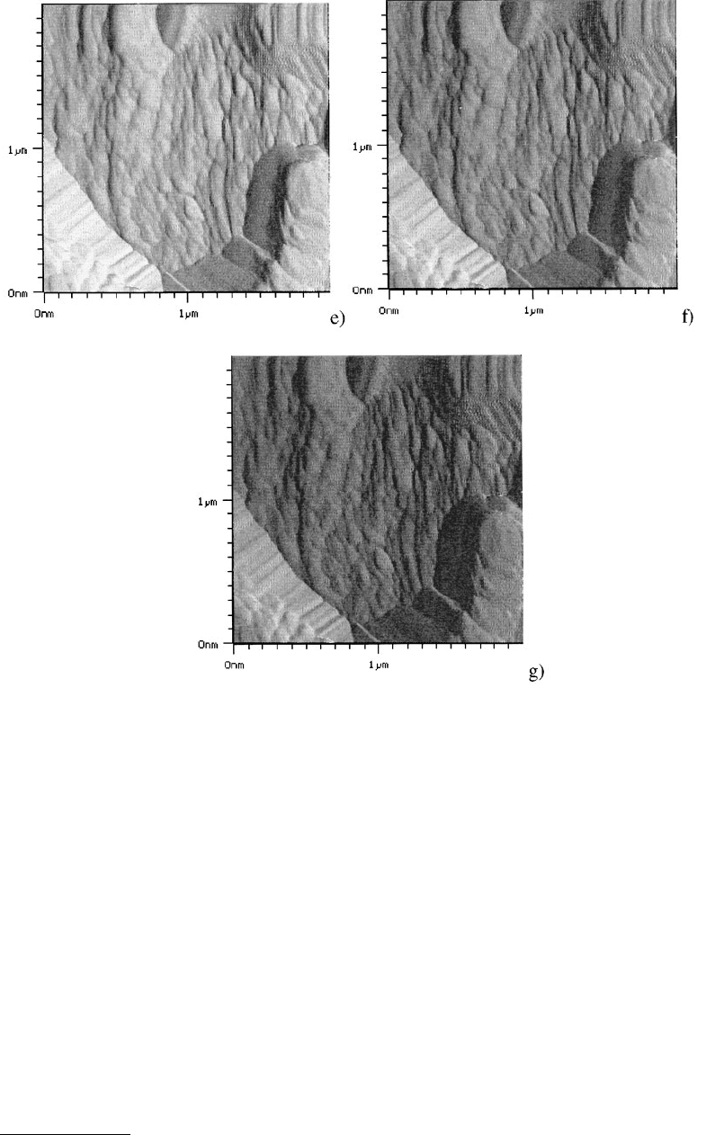
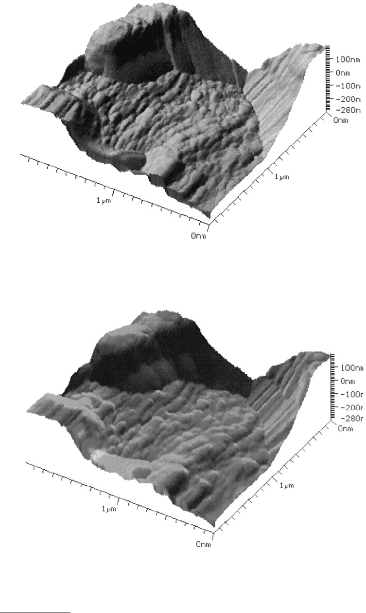
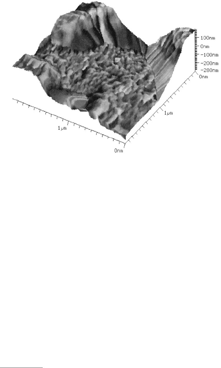
FIGURE 2.39 Illuminated surface: (a) shows an illumination from the top (0°) with an elevation of 50°. (b) is from

45° (upper right) — (b) and all the other illuminations have an elevation of 50°. (c) is at 90°, (d) at 135°, (e) at 180°,

(f) at 225°, (g) at 270°, and (h) at 315°.

In many force microscopes the scales can be calibrated rather accurately, for instance, using the procedure

outlined above, but the zero points are quite unreliable. The zeros usually do not drift very much, but

it is hard to determine their exact position on the force scales.

Figure 2.50 shows the two-dimensional histograms calculated with data from Figure 2.35. These his-

tograms, ﬁrst used as a data reduction means in communications with satellites (Yaroslavski, 1985), show

correlations between different data channels. In the case of friction data, the lateral force F

(x,y) and the

normal force F

(x,y) are used as an address to bins arranged in a two-dimensional array (Marti, 1993a,b;

Marti et al., 1993). For every data point (x,y) the bin addressed by (F

(x,y), F

(x,y)) is incremented by

one. The two-dimensional histogram then shows the statistical weight of every combination. For a

constant friction coefﬁcient and a varying normal force, one obtains (F

(x,y), F

(x,y)) pairs located on

a straight line, with the slope equal to the friction coefﬁcient. Since the creation of a two-dimensional

histogram is independent of the zero point values, it is not necessary to know the offsets. If different

materials are present on the sample surface and if they have friction coefﬁcients of sufﬁciently different

magnitudes, then the two materials will fall into different groups of bins in the two-dimensional histo-

gram. Displaying only points falling into one group of bins will select all the locations where one material

is present (Marti 1993a,b; Lüthi et al., 1995; Meyer et al., 1996).

FIGURE 2.40(a–d)

As was shown above, the two-dimensional histogram analysis is not limited to an analysis of friction

force data. It could be applied to other problems in scanning probe microscopy, for instance, relating

spectroscopic data to the tunneling current or to determine the locations of excessive forces or tunneling

currents, to name a few.

2.9.8 Some Common Image-Processing Methods

Since many commercial data acquisition systems use implicitly some kind of data processing, we will

describe some of the effects of these procedures. Since the original data is commonly subject to slopes

on the surface, most programs use some kind of slope correction. Figure 2.51 shows the effect of such

algorithms. In Figure 2.51a there is the original data, without any correction. The least disturbing way

is to subtract a plane z(x,y) = a

x + a

y + a

from the data. The coefﬁcients are determined by ﬁtting

z(x,y) to the data. As can be seen in Figure 2.51b, the main effect is to lower the right side and to lift up

the left side. A more severe option is to subtract a second order function such as ˜z(x,y) = a

+ a

xy + a

x + a

y + a

. Again, the parameters are determined with a ﬁt. This function is appropriate for

FIGURE 2.40 Inﬂuence of the elevation angle on the displayed data in illumination mode. The data are illuminated

from the right. (a) has an elevation angle of 0° (from top). (b) is at 15°, (c) at 30°, (d) at 45°, (e) at 60°, (f) at 75°,

and (g) at 90° (parallel to the surface).

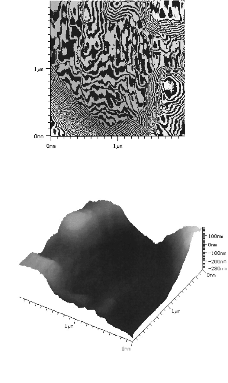
FIGURE 2.41 A discontinuous color table can generate a data display similar to contour maps. Here we have used

a color table with 32 steps.

FIGURE 2.42 Three-dimensional rendering of the data of Figure 2.35. The shading of the surface is purely topo-

graphical.

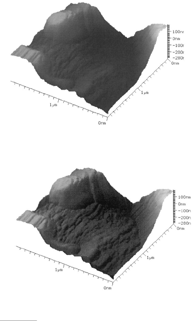
FIGURE 2.43 Three-dimensional rendering of the data of Figure 2.35. The shading of the surface is 80% topo-

graphical and 20% illumination.

FIGURE 2.44 Three-dimensional rendering of the data of Figure 2.35. The shading of the surface is 60% topo-

graphical and 40% illumination.

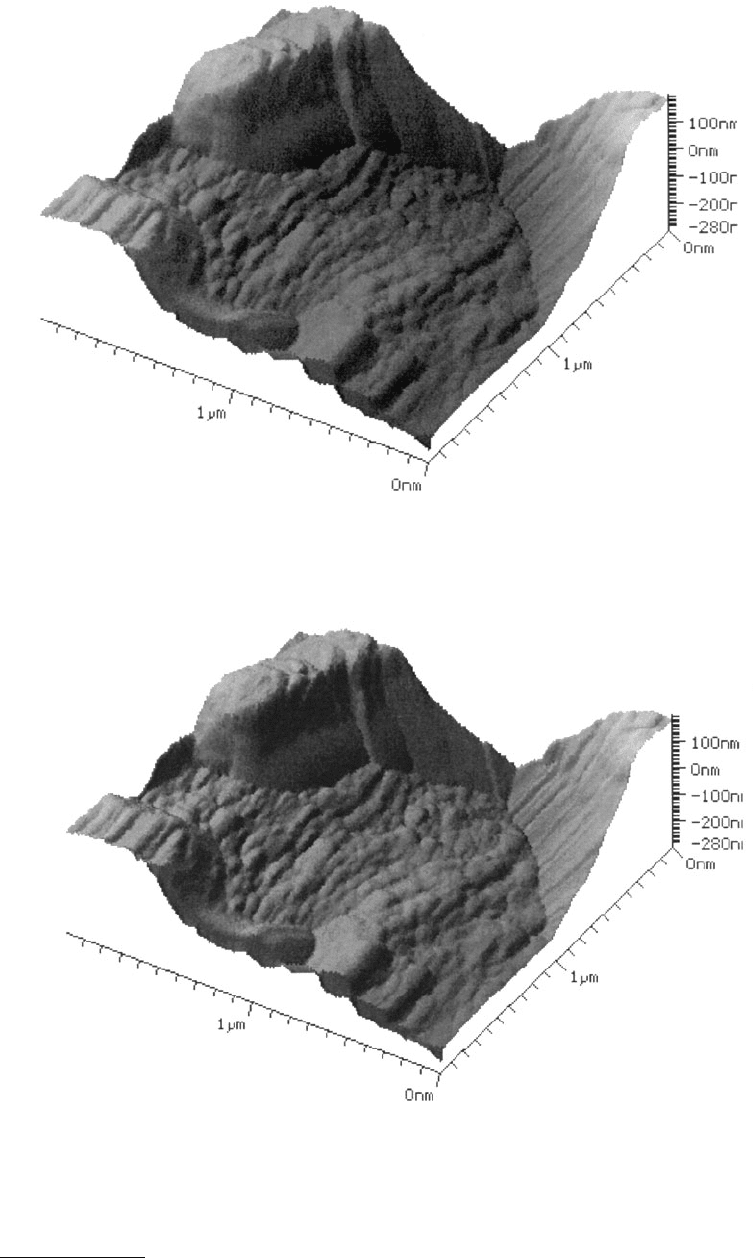
FIGURE 2.45 Three-dimensional rendering of the data of Figure 2.35. The shading of the surface is 40% topo-

graphical and 60% illumination.

FIGURE 2.46 Three-dimensional rendering of the data of Figure 2.35. The shading of the surface is 20% topo-

graphical and 80% illumination.

FIGURE 2.47 Three-dimensional rendering of the data of Figure 2.35. The shading of the surface is purely illumi-

nation.

FIGURE 2.48 Three-dimensional rendering of the data of Figure 2.35. The topography channel determines the

height, whereas the stiffness channel gives the color.

almost plane data, where the nonlinearity of the piezos caused such a distortion. It is obvious that the

data are now grossly distorted. Both algorithms have two disadvantages. They can only be used for data

that are already known and they can be calculation intensive.

During data acquisition, only part of the data is known. Therefore, other algorithms which only work

on single rows or columns are preferred. Figure 2.51d shows the effect of subtracting the average of a

row from every point in the row. Data sets that have ﬁne structure and no long-range variations of the

slope can safely be subject to this algorithm. These data, however, are affected and change its character.

Figure 2.51e shows the same procedure, but now applied to the columns. Figure 2.51f is an extension to

subtracting the data. Here not only the average value is subtracted, but also the slope of a line ﬁtted to

one row. Hence, all the tilt is also taken out of the data. This is a dangerous function, since it can

completely change the data appearance. However, most data acquisition programs use exactly this func-

tion. Figure 2.51g, ﬁnally, is the same procedure applied to rows.

Figure 2.51h shows the effect of an unsharp mask. This procedure ﬁrst calculates a low-pass ﬁltered

image by averaging all the points in the neighborhood and then subtracting this value. As can be seen,

the effect is a high-pass ﬁlter where all the slow variations are gone. While this technique is ideally suited

to ﬁnding out if there are short-range variations in the data.

With data sets such as that in Figure 2.35 where low-lying data are almost not visible, one might be

tempted to apply a technique widely used in image processing: histogram equalization (Figure 2.52).

This technique calculates a cumulative histogram of the z-values. The number as a function of the height

class deﬁnes a function. The inverse of this function is then applied to the data. After this operation the

histogram has an equal number of points in the height classes. Since it is a nonlinear function, we do

not recommend that it be used on AFM data.

FIGURE 2.49 Three-dimensional rendering of the data of Figure 2.35. The topography channel determines the

height, whereas the adhesion channel gives the color.