Blank B.E., Krantz S.G. Calculus: Single Variable

Подождите немного. Документ загружается.

59. By the demand curve for a given commodity, we mean

the set of all points ( p, q) in the pq2plane where q is the

number of units of the product that can be sold at price p.

The elasticity of demand for the product at price p is

deﬁned to be E( p) 52q

( p)  p/q( p).

a. Suppose that a demand curve for a commodity is

given by

p 1 q 1 2p

q 1 3pq

5 1000

when p is measured in dollars, and the quantity q of

items sold is measured by the 1000. For example, the

point ( p, q) 5 (6, 3.454) is on the curve. That means

that 3454 items are sold at $6. What is the slope of the

demand curve at the point (6, 3.454)?

b. What is elasticity of demand for the product of part

(a) at p 5 $6.

60. Let a be a positive constant. The Kulp Quartic is the

graph of the equation x

5 a

2 y

). Show that this

curve is also described by the parametric equations x 5 a

tan (t), y 5 a cos (t). Show that the Kulp Quartic is,

furthermore, the union of the graphs of two (explicit)

functions. Set a 5 2. Find the slope of the tangent line at

(2,

ﬃﬃﬃ

) by three different methods.

Computer/Calculator Exercises

c In each of Exercises 6164, a curve is given as well as an

abscissa x

. Find the ordinate y

such that (x

, y

) is on the

curve, and determine the slope of the tangent line to the curve

at (x

, y

). b

61. x

2 3xy 1 y

5 0 x

5 10.000

62. x

2 y

5 0, x6¼yx

5 3.0000

63. x

2 x

1 y

5 0 x

521.4649

64. ln (xy) 1 y 5 5 x

5 2.124

c In each of Exercises 6568, a curve is given as well as an

abscissa x

. Find the ordinate y

such that (x

, y

) is on the curve,

and determine the equation of the tangent line to the curve at

, y

). b

65. x

2 2xy 1 y

5 0 x

5 10.000

66. x

2 y

5 0, x 6¼yx

5 3.1416

67. x

2 x

1 y

5 0 x

522.0125

68. e

1 y 5 10 x

5 1.5727

c In Exercises 6972, plot the given curve in a viewing

rectangle

that contains the given point P

. Then add a plot of

the tangent line to the curve at P

. b

69. x

2 2xy 1 y

5 0 P

5 (0.5, 0.9304 ...)

70. x

2 y

5 0, x 6¼yP

5 (3.7500, 2.0860)

71. x

2 x

1 y

5 0 P

5 (2.1125, 1.9289)

72. xe

1 y 5 2 P

5 (1.0000, 0.44285)

Implicit Differentiation

c In Exercises 7377, plot the given parametric curve x 5 ϕ

(t), y 5 ϕ

(t) in a viewing rectangle that contains the given

point P

. Find the equation of the tangent line at P

. Add the

tangent line to your plot. b

73. ϕ

(t) 5 8 cos (t), ϕ

(t) 5 8 sin (t)(sin (t/2))

5 (4,

ﬃﬃﬃﬃﬃﬃﬃ

ð3Þ

(Tear Drop Curve)

74. ϕ

(t) 5 100t/(1 1 t

)

, ϕ

(t) 5 100t

/(1 1 t

)

5 (32, 16) (t 5 1/2) (Regular Bifolium)

75. ϕ

(t) 5 (1 1 t

)/(1 1 3t

), ϕ

(t) 5 4t/(1 1 3t

5 (1/2, 1) (t 5 1)

76. ϕ

(t) 5 (32t

)/(1 1 t

), ϕ

(t) 5 2t(3 2 t

)/(1 1 t

5 (1, 2) ( t 5 1/2) (Maclaurin’s Trisectrix)

77. ϕ

(t) 5 1 2 3t

, ϕ

(t) 5 t 2 3t

5 (1/4,21/8) (t 521/2) (Cubic of Tschirnhaus)

78. Graphically locate the points on the curve x

1 x 1

5xy

5 1 where the tangent line is vertical. Conﬁrm that

the method of implicit differentiation yields the same

points.

79. Graphically locate the points on the curve x

26xy

5 4

where the tangent line is vertical. Conﬁrm that the

method of implicit differentiation yields the same points.

80. Plot the ampersand curve

ðx

2 y

Þðy 2 1Þð2y 2 3Þ 52ðx

2 2yÞ

in the viewing window [23/2, 3/2] 3 [21/4, 3/2]. Notice

that P

5 (1, 1) lies on the ampersand. However, the

general formula for dy/dx at P

results in the meaning-

less 0/0. This complication is not surprising: we expect

some unusual behavior at P

because the ampersand has

two tangent lines at P

, as is evident from the plot. Find

points P

5 (x

, 0.9999) and P

5 (x

, 0.9999) on the

ampersand with 0 , x

, 1 and 1 , x

. Calculate the

slopes m

and m

of the tangent lines at P

and P

.As

approximations to the two tangent lines at P

, add to your

plot the two lines passing through P

with slopes m

and m

81. Let q( p) be the demand function of Exercise 59a. Use the

method of implicit differentiation to ﬁnd q

(4). Find q

(4.2) and q (3.8). Use these values to approximate q

(4).

82. Saha’s equation describes the degree of ionization within

stellar interiors. For our own sun,

1 2 y

0:787 3 10

expð158000=xÞ

3=2

where y represents the fraction of ionized atoms in the

sun, and x represents solar temperature in degrees Kelvin.

Find dy/dx when x 5 63 10

3.8 Implicit Differentiation 245

3.9 Differentials and Approximation of Functions

Loosely interpreted, the equation

ðcÞ5 lim

Δx-0

f ðc 1 ΔxÞ2 f ð cÞ

Δx

says that

ðcÞ

f ðc 1 Δ x Þ2 f ðcÞ

Δx

ð3:9:1Þ

when Δx is small and nonzero. A choice of a fairly small value of Δx often gives a

good approximation. With a little algebraic manipulation, we can convert approx-

imation (3.9.1) into an approximation of f (c 1 Δx):

f ðc 1 ΔxÞf ðcÞ1 f

ðcÞΔx: ð3:9:2Þ

We may interpret equation (3.9.2) as follows: If we know the values of f (c) and f

(c),

then we can estimate the value of f (x ) at a nearby point x 5 c 1 Δx. In this context,

the point c is sometimes called a base point. When Δx can take any value in an

interval (2h, h), so that x 5 c 1 Δx can take any value in ( c2h, c1h), we refer to c as

the center of approximat ion (3.9.2). Sometimes we abbreviate f (x 1 Δx) 2 f (x)as

Δf (x). Notice that Δf (x) is the increment in the functional value when the inde-

pendent variable x is incremented by Δx. Using this notation and replacing c with x,

approximation (3.9.2) becomes

Δf ðxÞf

ðxÞΔx; ð3:9:3Þ

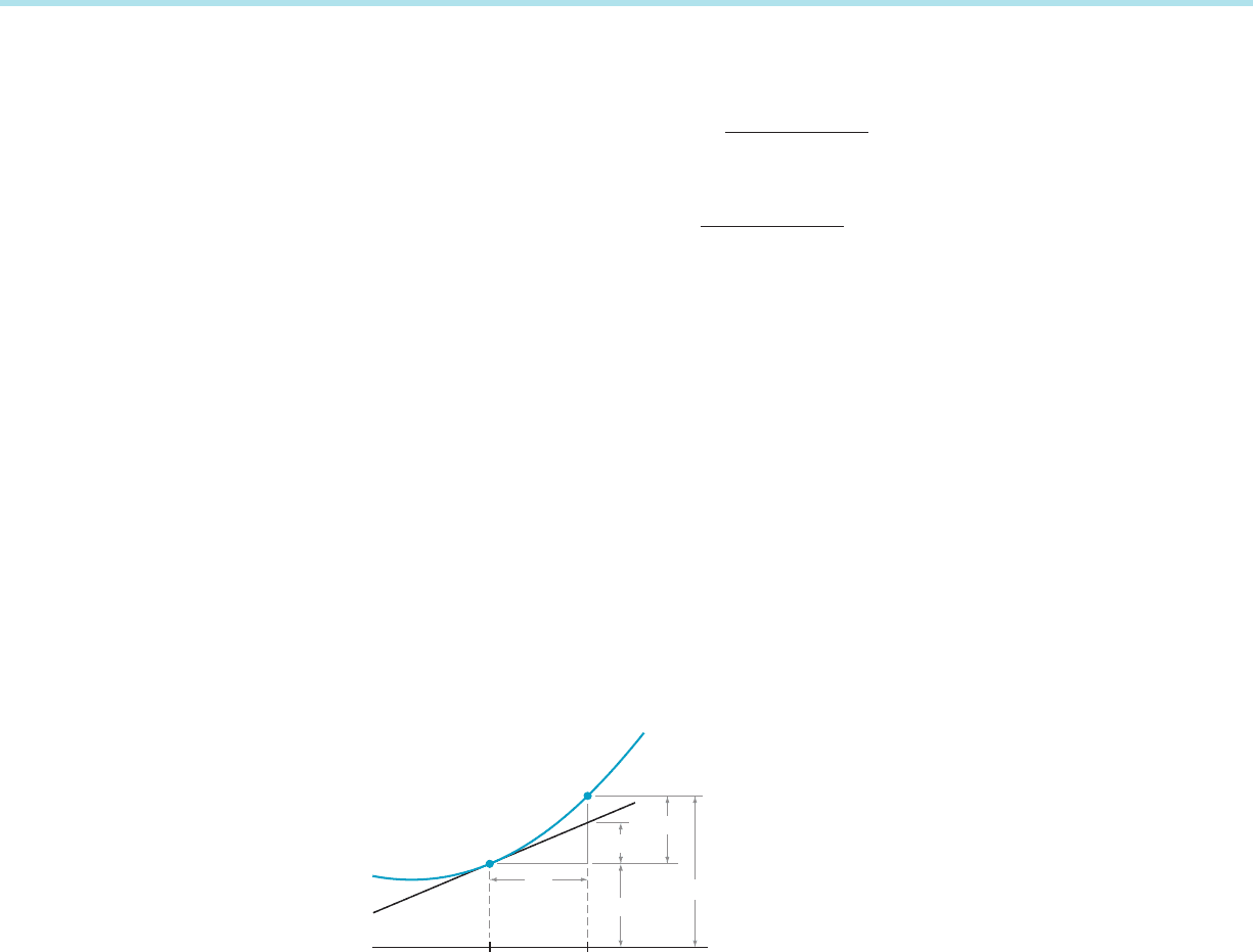
which is illustrated in Figure 1. We call this approxi mation scheme the method of

increments.

⁄ EX

AMPLE 1 Use approximation (3.9.2) to estimate the value of

ﬃﬃﬃﬃﬃﬃﬃ

4:1

Solution To

make the left side, f (c1Δx), of approximation (3.9.2) equal to the

quantity

ﬃﬃﬃﬃﬃﬃﬃ

4:1

that we are to approximate, we set f (x) 5 x

1/2

and c 1 Δx 5 4.1. We

calculate f

(x) 5 (1/2) x

21/2

. We must now select two numbers c and Δx that sum to

4.1. If we choose c 5 4 and Δx 5 0.1, then f (c) 5 4

1/2

5 2, f

21/2

5 1/4,

and approximation (3.9.2) becomes

(c, f (c))

f(c)x

x

f(c)

f(c)

f(c  x)

(c  x, f(c  x))

c  xc

m Figure 1 f ðc 1 Δ xÞ2 f ðcÞ5 Δf ðcÞf

ðcÞΔx

246 Chapter 3 The Derivative

ﬃﬃﬃﬃﬃﬃﬃ

4:1

5 f ðc 1 ΔxÞf ðcÞ1 f

ðcÞΔx 5 2 1

ð0:1Þ5 2:025:

A calculator shows that our simple approximat ion is accurate to within 0.001.

INSIGHT

The selection of c 5 4 in Example 1 is no accident. It is easy for us to

evaluate f and f

at this particular c. Moreover, c 5 4 is near to 4.1, which means that Δx

is small. Making Δx small tends to increase accuracy. If, for example, we apply the

method of increments to estimate

ﬃﬃﬃﬃﬃ

using the same choice of c as in Example 1,

namely c 5 4, then Δx 5 6, and we obtain

ﬃﬃﬃﬃﬃ

 4

1=2

1 ð1=2Þ4

21=2

ð6Þ5 3:5: The true

value of

ﬃﬃﬃﬃﬃ

is 3:162:::. Our approximation is therefore off by more than 0.33. A much

better estimate is obtained by taking c 5 9 and Δx 5 1. The resulting approximation is

ﬃﬃﬃﬃﬃ

 9

1=2





21=2

ð1Þ5 3:166:::;

which is correct to two decimal places. The accuracy of the method of increments

strongly depends on the size of the increment Δx. In general, the smaller the increment,

the more accurate the approximation.

⁄ EXAMPLE 2 A machine shop builds triangular jigs of isosceles shape. The

bases are precut and have length exactly 10 inches. The heights vary. During a rush

period, the measurement of the two sides gets sloppy, and they are off by as much

as 0.1 inch. By about how much will the area of the resulting jig deviate from the

desired area?

Solution The

ideal length of the two equal sides is denoted by ‘ in Figure 2. The

height of the triangle is h 5

ﬃﬃﬃﬃﬃﬃﬃﬃﬃﬃﬃﬃﬃﬃ

‘

2 5

, and the area is therefore

Að‘Þ5

 10  h 5 5 

ﬃﬃﬃﬃﬃﬃﬃﬃﬃﬃﬃﬃﬃﬃﬃ

‘

2 25

Notice that A

ð‘Þ5 5‘ð‘

225Þ

21=2

: If the length measurement is off by Δ‘, then the

area is

Að‘ 1 Δ‘ÞAð‘Þ1 A

ð‘ÞΔ‘ 5 Að‘Þ1 5‘ ð‘

225Þ

21=2

 Δ‘:

The increment in area is therefore

ΔA  Að‘ 1 Δ‘Þ2 Að‘Þ5‘ ð‘

225Þ

21=2

 Δ‘:

Because |Δ‘| # 0.1, the approximate deviation ΔA of the area can be as much as

5‘ (‘

2 25)

21/2 

0.1, or

‘

ﬃﬃﬃﬃﬃﬃﬃﬃﬃﬃﬃﬃﬃﬃﬃ

‘

2 25

For example, if the desired length ‘ is 20 inches, then we substitute ‘ 5 20 into

this formula and ﬁnd that the error in area is approximately 0.5164 in

. ¥

INSIGHT

In Example 2, the error in area can be found from the area equation

Að‘Þ5 5

ﬃﬃﬃﬃﬃﬃﬃﬃﬃﬃﬃﬃﬃﬃﬃ

‘

2 25

. Thus,

error in area 5 Að‘ 1 0:1Þ2 Að‘Þ5 5

ﬃﬃﬃﬃﬃﬃﬃﬃﬃﬃﬃﬃﬃﬃﬃﬃﬃﬃﬃﬃﬃﬃﬃﬃﬃﬃﬃﬃﬃﬃ

ð‘ 1 0:1Þ

2 25

2 5

ﬃﬃﬃﬃﬃﬃﬃﬃﬃﬃﬃﬃﬃﬃﬃ

‘

2 25

h  ᐉ

 5

ᐉᐉ



m Figure 2

3.9 Differentials and Approximation of Functions 247

However, this formula for the error does not allow us to easily understand the dependence

on ‘. The important feature of the method of increments in Example 2 is that it yields a

simple formula that works for all triangles under consideration with a minimum of

calculation.

Increments in

Economics

If we take Δx 5 1 in (3.9.2), then we obtain f (c 1 1) f (c) 1 f

(c)or

f ðc 1 1Þ2 f ðcÞf

ðcÞ: ð 3 :9:4Þ

This approximation is often used in economics. For example, if f (x ) represents the

quantity of goods produced as a function of the amount x of labor, then f is called

the product of labor. The increment in production that is achieved by adding one

more unit of labor is known as the marg inal product of labor (MPL). Thus

MPLðcÞ5 f ðc 1 1Þ2 f ðcÞ:

If we compare this deﬁnition of MPL with approximation (3.9.4), then we obtain

MPLðcÞf

ðcÞ:

Many economics texts deﬁne MPL(c)tobef

that is typically found in textbooks about macroeconomics.

Another example of this construction is marginal cost. If C(x) is the cost of

producing x units of an item, then the marginal cost is the cost C(x 1 1) 2 C(x)of

producing one more item. In practice, the approximation C

(x) is generally used

instead of C(x 1 1) 2 C(x). Similarly, if R(x)andP(x) are the revenue and proﬁt,

respectively, produced by selling x items, then R

(x)andP

(x) are the marginal

revenue and marginal proﬁt, respectively.

Linearization Let’s look at the approximation (3.9.2) again. If we let x 5 c 1 Δx, then we get

f ðxÞ5 f ðc 1 Δx Þf ðcÞ1 f

ðcÞΔx 5 f ðcÞ1 f

ðcÞðx 2 cÞ

f ðxÞf ðcÞ1 f

ðcÞðx 2 cÞð3:9:5Þ

for x close to c. The right hand side of this approximation is a function of x which

we will denote by L:

LðxÞ5 f ðcÞ1 f

ðcÞðx 2 cÞ: ð3:9:6Þ

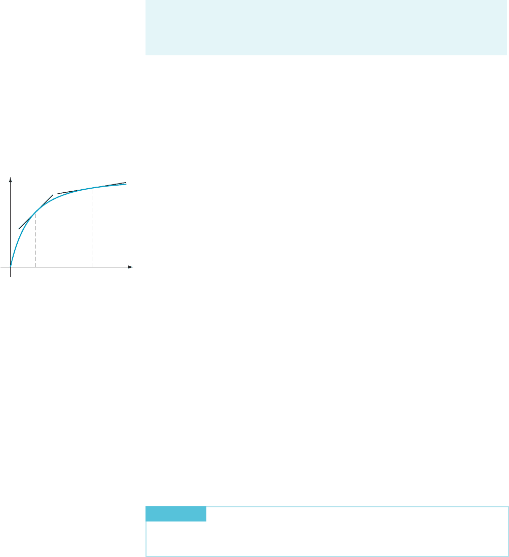
Notice that the graph of L is the tangent line to the graph of f at (c, f (c)).

DEFINITION

The function L deﬁned by (3.9.6) is said to be the linearization of

f at c. The approximation L(x) f (x) for x close to c is called the tangent line

approximation to f at c. Sometimes the term best linear approximation is used.

In the leftmost viewing window of Figure 4 we see the graph of a function f

together with its linearization at c. We have zoomed in around the point (c, f (c)) in

the middle view. Notice how good an approximation L is of f in this viewing

m Figure 3 Level of output as a

function of the quantity of labor

input. The slope of the tangent

line equals the marginal product

of labor.

248 Chapter 3 The Derivative

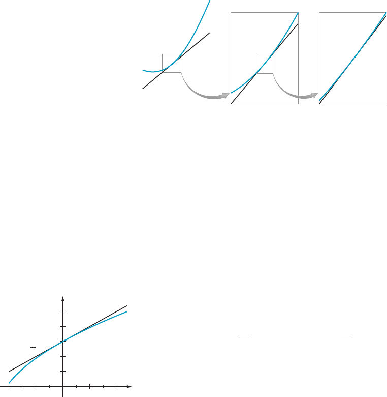
window. In the right view, we have zoomed in still further. Distinguish between L

and f. There is, to be sure, a difference between these two functions—it is just too

minute to show up on screen.

Important

Linearizations

It is useful to know certain linearizations because of the frequency with which they

occur in calculus an d other subjects.

⁄ EX

AMPLE 3 Show that

ð11xÞ

 1 1 p  x

for values of x near 0.

Solution Let f (x) 5 (11x)

and c 5 0. Using the Chain RulePower Rule, we have

ðxÞ5

ð11xÞ

5 pð11xÞ

p21

ð1 1 xÞ5 pð11xÞ

p21

Therefore f

(0) 5 p (1 1 0)

p21

5 p. Approximation (3.9.5) takes the form

ð11xÞ

5 f ðxÞf ðcÞ1 f

ðcÞðx 2 cÞ5 1 1 p ðx 2 0Þ5 1 1 p  x;

as required. Figure 5 illustrates the approximation when p 5 1/2.

⁄ EXAMPLE 4 Show that the linearizations of sin (x), cos (x), and tan (x)at

x 5 0 are

sinðxÞx; cosðxÞ1; and tanðxÞx

Solution Let c 5 0.

For f (x) 5 sin (x), approximation (3.9.5) becomes

sinðxÞ5 f ðxÞf ðcÞ1 f

ðcÞðx 2 cÞ5 sinð0Þ1 cosð0Þðx 2 0Þ5 x:

Similarly, for f (x) 5 cos (x), approximation (3.9.5) becomes

cosðxÞ5 f ðxÞf ðcÞ1 f

ðcÞðx 2 cÞ5 cosð0Þ1 sinð0Þðx 2 0Þ5 1

Finally, for f (x) 5 tan ( x ), we have

tanðxÞ5 f ðxÞf ðcÞ1 f

ðcÞðx 2 cÞ5 tanð0Þ1 sec

ð0Þðx 2 0Þ5 x: ¥

m Figure 4

y  (1  u)

12

0.4 0.80.8 0.4

0.6

0.8

1.2

1.4

y  1 

m Figure 5

3.9 Differentials and Approximation of Functions 249

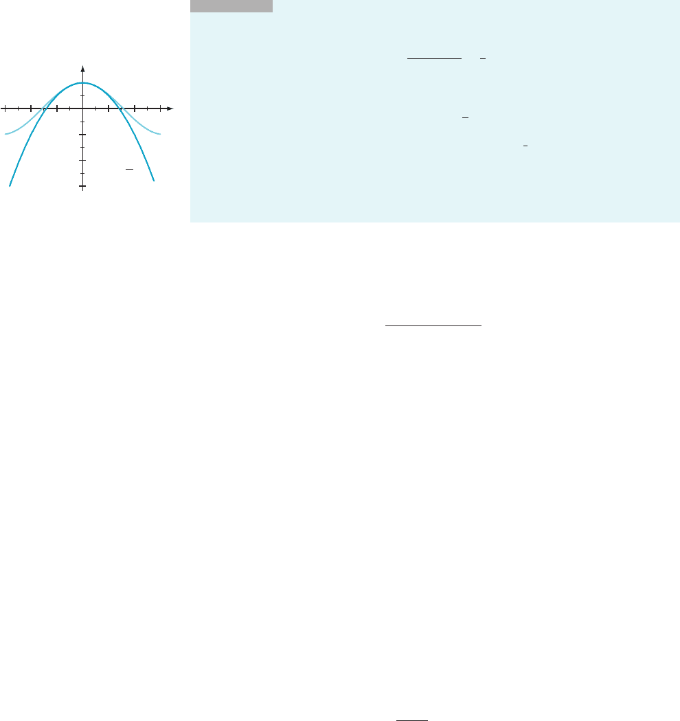
INSIGHT

It should be noticed that we have already obtained an estimate that is

more precise than the linearization cos (x) 1. Recall the basic limit formula:

lim

x-0

1 2 cosðxÞ

that we derived in Section 2.3. This limit says that

cosðxÞ1 2

for small x. The two functions f (x) 5 cos (x) and g(x) 5 1 2

have been graphed in

Figure 6. Notice how well g approximates f for small values of x—but only for small

values of x. Clearly this approximation of cos (x) is better than the linearization L(x) 5 1.

In Chapter 10, we will learn a general approach, called the Taylor expansion, for

obtaining estimates that are more precise than the tangent line approximation.

Differentials In the early days of calculus, the ideas were not made precise. There was no concept

of “limit.” Instead, the derivative was obtai ned as a quotient of inﬁnitesimally small

quantities:

f ðx 1 dxÞ2 f ðxÞ

Here dx represents a quantity that is positive but smaller than every positive real

number. What does this mean? Nobody really knew. Nevertheless, calculations of

derivatives of speciﬁc functions were done with these mysterious quantities. Many

times these calculations involved strange steps that could not be rigorously justiﬁed.

It took nearly 200 years for the puzzling theory of differentials (which is

what we call expressions like “dx”) to be replaced by the more precise notions

of increment and limit. More recently, in 1960, it was determined that the notion of

differential could be made precise. However, the modern theory of inﬁnitesimals is

a subject for an advanced course in mathematical logic, and we cannot discuss it

here. What you need to know is that the notation of differentials is still used today,

purely as an intuitive device. It is reassuring to know that differentials can be

treated rigorously, but for us, they will be just an economical way to express the

method of increments. Here is how we do it.

As Δx becomes smaller in (3.9.3), the estimate becomes more accurate. When

Δx becomes “inﬁnitesimal,” estimate (3.9.3) becomes an equality. We represent

the inﬁnitesimal increment in x as dx and the resulting inﬁnitesimal change in f as

df. Thus (3.9.3) becomes

df ðxÞ5 f

ðxÞdx: ð3:9:7Þ

It is tempting to divide this equation through by dx to yield the identity

df ðxÞ

5 f

ðxÞ:

This explains the origin of the Leibniz notation for the derivative. But, for our

purposes, we think of equation (3.9.7) as nothing more than another way to write

approximation (3.9.3). Indeed, formula (3.9.7) is sometimes referred to as a

differential approximation.

3 13

cos(x)

1

1 

2

3

m Figure 6

250 Chapter

3 The Derivative

b ALOOKBACK It may help to remember that there is only one key idea behind all

the terminology that has been introduced. Linearization, best linear approximation,

tangent line approximation ,anddifferential approximation all refer to the same

thing: If f is differentiable at c, if the point (x, y) is on the tangent line to the graph

of f at (c, f (c)), and if x is close to c, then y is close to f (c).

We conclude by stating the rules of differentiation in differential form. In the

following table, c repres ents a constant.

dðcÞ 5 0 dðsinðuÞÞ 5 cosðuÞdu

dðcuÞ 5 cdðuÞ dðcosðuÞÞ 52sinðuÞdu

dðu 1 υÞ 5 du 1 dυ dðtanðuÞÞ 5 sec

ðuÞdu

dðuυÞ 5 udυ 1 υdu dðsecðuÞÞ 5 secðuÞtanðuÞdu

dðu=υÞ 5 ðυdu 2 udυÞ=v

dðcotðuÞÞ 52csc

ðuÞdu

dð1=υÞ 52dυ=υ

dðcscðuÞÞ 52csc ðuÞcotðuÞdu

dðu

Þ 5 pu

p21

du dðexpðuÞÞ 5 expðuÞdu

dðlnðuÞÞ 5 ð1=uÞdu dða

Þ 5 a

lnðaÞdu

QUICK QUIZ

1. Use differentials to approximate 7.9

1/3

2. What is the linearization of cos (x) 1 sin (x)at0?

3. What is the best linear approximation of f (x) 5 ln(11x)atx 5 0?

4. What is the differential approximation of f (x) 5 e

Answers

1. 21(1/3

) 8

22/3

(20.1) 2. 11x 3. x 4. e

EXERCISES

Problems for Practice

c In Exercises 124, use the method of increments to esti-

mate the value of f (x) at the given value of x using the known

value f (c). b

1. f (x) 5

ﬃﬃ

ﬃ

; c 5 4, x 5 3.9

2. f (x) 5

ﬃﬃﬃ

; c 5 9, x 5 8.95

3. f (x) 5 1/x

1/3

, c 5 8, x 5 8.07

4. f (x) 5 x

23/2

, c 5 4, x 5 4.21

5. f (x) 5 x

2/3

, c 5 8, x 5 8.15

6. f (x) 5 (11x)

21/4

, c 5 15, x 5 16

7. f (x) 5 (1 1 7x

2)1/3

, c 5 3, x 5 2.8

8. f (x) 5 sin (x), c 5 0, x 5 0.02

9. f (x) 5 cos (x), c 5 π/3, x 5 1.06

10. f (x) 5 sin (x) 2 cos (x),c 5 π/4, x 5 0.75

11. f (x) 5 tan (x), c 5 π/4, x 5 0.8

12. f (x) 5 cot (x), c 5 π/3, x 5 1

13. f (x) 5 sec (x), c 5 π/6, x 5 0.5

14. f (x) 5 csc

(πx/4), c 5 1, x 5 0.94

15. f (x) 5 ln (x), c 5 e

, x 5 20

16. f (x) 5 x ln (x), c 5 1, x 5 0.92

17. f (x) 5 e

, c 5 0, x520.17

18. f (x) 5 xe

, c 5 0, x 5 0.12

19. f (x) 5 16

, c 5 0, x 5 0.13

20. f (x) 5 x

, c 5 0, x 5 0.15

21. f (x) 5

ﬃﬃﬃ

cos (π/(x 1 3)), c 5 1, x 5 0.81

22. f (x) 5 sinð

ﬃﬃﬃﬃﬃﬃ

πx

Þ, c 5 π/16, x 5 0.2

23. f (x) 5 sin

(x), c 5 π/4, x 5 0.75

24. f (x) 5

ﬃﬃﬃ

=ð1 1

ﬃﬃﬃ

Þ, c 5 9, x 5 8.6

c In Exercises 2530, choose an appropriate function f and

point c,

and use the differential approximation of f in order to

estimate the given number. Compute the absolute error. b

25.

ﬃﬃﬃﬃ

ﬃ

26.

ﬃﬃﬃﬃﬃﬃﬃﬃﬃﬃﬃﬃ

2 7:5

27.

ﬃﬃﬃﬃﬃﬃﬃﬃﬃﬃﬃﬃﬃﬃﬃﬃﬃﬃ

1 1

ﬃﬃﬃﬃﬃﬃﬃ

9:7

3.9 Differentials and Approximation of Functions 251

28. sin (0.48π)

29. cos (55



)

30. tan (0.23π)

c In Exercises 3136, calculate the linearization L(x) 5

f (0)1f

(0) x for the given function f at c 5 0. b

31. f (x) 5 1/(3 1 2x)

32. f (x) 5 x

ﬃﬃﬃﬃﬃﬃﬃﬃﬃﬃ

ﬃ

1 1 x

33. f (x) 5 x/(41x)

3/2

34. f (x) 5 x/e(x)

35. f (x) 5 1/(x 1 cos (x))

36. f (x) 5 cos (x)/(1 1 sin (2x))

c In Exercises 3742, calculate the linearization L(x) 5 f (c)1

(c), (x2c) for the given function f at the given value c. b

37. f (x) 5 cos

(x), c 5 π/3

38. f (x) 5 tan (x), c 5 π/4

39. f (x) 5 (25/9)

, c 5 1/2

40. f (x) 5 x ln (x), c 5 e

41. f (x) 5 e(x 2 1)/x, c 5 1

42. f (x) 5 cos

(x),c 5 π/4

Further Theory and Practice

43. Suppose that a, b, and p are constants. What is the line-

arization of f (x) 5



11ax

11bx



at 0?

44. Suppose that f, g, and h are differentiable functions and

that f 5 g  h. Suppose that g(4) 5 6, dg(4) 5 7, dx, h(4) 5

5, and dh(4) 522dx. What is df(4)?

45. Explain how the linearizations of the differentiable

functions f and g at c may be used to discover the product

rule for ( f g)

(c).

46. Explain how the linearizations of the differentiable func-

tions f and g at c may be used to discover the quotient rule

for ( f/g)

Suppose that (u, υ)/ F(u, υ) is a given function of two

variables. Suppose that y is an unknown function of x that

satisﬁes the differential equation y

(x) 5 F(x, y(x)) and initial

condition y(x

) 5 y

. (Together these two equations con-

stitute an initial value problem. We will study such problems

in greater detail in Chapter 7.) The method of increments

canbeusedtoapproximatey(x

)wherex

5 x

1Δx:

yðx

Þyðx

Þ1 y

ðx

ÞΔx 5 y

1 Fðx

; y

ÞΔx

|ﬄﬄﬄﬄﬄﬄﬄﬄﬄﬄﬄﬄﬄ{zﬄﬄﬄﬄﬄﬄﬄﬄﬄﬄﬄﬄﬄ}

c We call this Euler’s Method of approximating the

unknown function y. In each of Exercises 4750, an initial

value

problem is given. Calculate the Euler’s Method

approximation y

of y(x

). b

47. dy/dx 5 x1y, y(1) 5 2, x

5 1.2

48. dy/dx 5 x2y, y(22) 521, x

522.15

49. dy/dx 5 x

2 2y, y(0) 5 3, x

5 1/4

50. dy/dx 5 11y/x, y(2) 5 1/2, x

5 3/2

c By the demand

curve for a given commodity, we mean the

set of all points ( p, q) in the pq plane where q is the number

of units of the product that can be sold at price p. In Exercises

5154 use the differential approximation to estimate the

demand q( p)

for a commodity at a given price p. b

51. Suppose

that a demand curve for a commodity is given by

p 1 q 1 2p

q 1 3pq

5 1000

when p is measured in dollars and the quantity q of items

sold is measured by the 1000. The point ( p

, q

) 5

(6.75, 3.248) is on the curve. That means that 3248 items are

sold at $6.75. What is the slope of the demand curve at the

point (6.75, 3.248)? Approximately how many units will be

sold if the price is increased to $6.80? Decreased to $6.60?

52. Suppose that a demand curve for a commodity is given by

q 1 p

ﬃﬃﬃ

=100 5 500005

when p is measured in dollars. This tells us that about

10000 units are sold at $5. Approximately how many units

of the commodity can be sold at $5.25? At $4.75?

53. The demand curve for a commodity is given by

190950

1 q

ﬃﬃﬃ

5 8019900

when p is measured in dollars. Use the differential

approximation to estimate the number of units that can

be sold at $9.75.

54. The demand curve for a commodity is given by

1 5p

ﬃﬃﬃ

5 39000

when p is measured in dollars. Approximately how many

units of the commodity can be sold at $1.80?

Calculator/Computer Exercises

c In each of Exercises 5558 a function f, a point c,an

increment Δx, and a positive integer n are given. Use the

method of increments to estimate f (c 1 Δx). Then let h 5 Δx/

N. Use the method of increments to obtain an estimate y

f (c 1 h). Now, with c 1 h as the base point and y

as the value

of f (c 1 h), use the method of increments to obtain an esti-

mate y

of f (c 1 2h). Continue this process until you obtain an

estimate y

of f (c 1 N h) 5 f (c 1 Δx). We say that we have

taken N steps to obtain the approximation. The number h is

said to be the step size. Use a calculator or computer to

evaluate f (c 1 Δx) directly. Compare the accuracy of the one-

step and N-step approximations. b

55. f (x) 5 x

1/3

, c 5 27, Δx 5 0.9, N 5 3

56. f (x) 5

ﬃﬃﬃ

, c 5 4, Δx 5 0.5, N 5 5

252 Chapter 3 The Derivative

57. f (x) 5 ln (x), c 5 e, Δx 5 32e, N 5 2

58. f (x)1=

ﬃﬃﬃ

, c528, Δx 5 1, N 5 4

c In each of Exercises 5962, an initial value problem is

given,

along with its exact solution. (Read the instructions for

Exercises 4750 for terminology.) Verify that the given

solution is correct by substituting it into the given differential

equation and the initial value condition. Calculate the Euler’s

Method approximation y

5 y

1F(x

, y

)Δx of y(x

) where

Δx 5 x

2 x

. Let m

5 (F(x

, y

) 1F(x

, y

))/2 and z

5 y

Δx. This is the Improved Euler Method approximation of

y(x

). Calculate z

. By evaluating y(x

), determine which of

the two approximations, y

or z

, is more accurate. b

59. dy/dx 5 x1y, y(1) 5 2, x

5 1.2; Exact solution: y(x) 5

4 exp (x 2 1) 2 x 2 1

60. dy/dx 5 x2y, y(22) 521, x

522.15; Exact solution:

y(x) 5 2 exp (222x)1x 2 1

61. dy/dx 5 x

2 2y, y(0) 5 3, x

5 1/4; Exact solution: y(x) 5

/22x/2 1 1/4 1 11/4 exp (22x)

62. dy/dx 5 11y/x, y(2) 5 1/2, x

5 3/2; Exact solution: y(x) 5

x ln (x)1x(1/4 2 ln (2))

c In each of Exercises 6365, a demand curve is given. Use

the

method of implicit differentiation to ﬁnd dq/dp. For the

given price p

, solve the demand equation to ﬁnd the corre-

sponding demand q

. Then use the differential approximation

with base point p

to estimate the demand at price p

. Find

the exact demand at price p

. What is the relative error that

results from the differential approximation? b

63. p

q 1 2pq

1/4

5 250100, p

5 5.10, p

5 5

64. 2 pq1pq

1/3

5 , 160200, p

5 9.75, p

5 10

65. p

q/10 1 5pq

1/5

5 1280200, p

5 1.80, p

5 2

3.10 Other Transcendental Functions

Exponential functions, logarithm functions, and trigonometric functions belong to

a large class of functions whose members are known as transcendental functions in

the mathematical literature. The functions we introduce in this section—inverse

trigonometric functions and hyperbolic functions—also belong to that class. With

these additions, we complete the list of transcendental functions that traditionally

receive detailed coverage in a ﬁrst-year calculus course. Students who pursue

further courses in quantitative subjects will encounter many other trans cendental

functions that arise in advanced classes or specialized studies.

Inverse Trigonometric

Functions

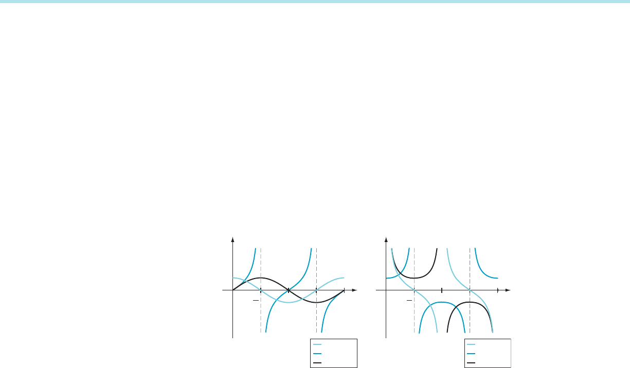
Figure 1 shows the graphs of the six trigonometric functions. Notice that each graph

has the property that some horizontal line intersects the graph at least twice.

Therefore no trigonometric function is invertible. Another way of seeing this point

is that each trigonometric function f satisﬁes the equation f (x 1 2π) 5 f (x) and is

therefore not one-to-one.

y  cos(x)

y  tan(x)

y  sin(x)

y  cot(x)

y  sec(x)

y  csc(x)

m Figure 1

3.10 Other Transcendental Functions 253

We must restrict the domains of the trigonometric functions if we want to

discuss inverses for them. In this section, we learn the standard metho ds for per-

forming this restriction operation. As you read this section, you may ﬁnd it useful to

refer back to Section 1.6 to review the properties of the trigonometric functions.

Inverse Sine and

Cosine

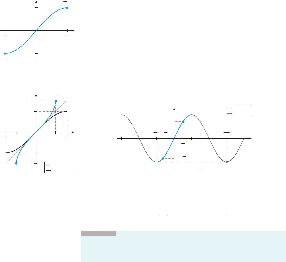
Consider the sine function with domain restricted to the interval [2π/2, π/2]. We

will denote this restricted function by x / Sin(x) (capitalized to emphasize that its

domain differs from that of the ordinary sine function). The graph of y 5 Sin(x)in

Figure 2 shows that x / Sin( x ) is a one-to-one function from [2π/2, π/2] onto

[21, 1]. Therefore it is invertible. Its inverse function, Sin

:[21, 1] - [2π/2, π/2],

is increasi ng, one-to-one, and onto. The exp ression Sin

(x) is read as ‘the inverse

sine of x” or “the arcsine of x” and is often denoted by arcsin (x). We can obtain

the graph of y 5 arcsin (x) by reﬂecting the graph of y 5 sin (x) in the line y 5 x

(Figure 3).

⁄ EX

AMPLE 1 Calculate arcsin ð

ﬃﬃﬃ

=2Þ, arcsin ð2

ﬃﬃﬃ

=2Þ, and arcsin

ðsinð3π=2ÞÞ.

Solution To

calculate arcsin (t), we look for the s A [2π/2, π/2] for which t 5 sin (s).

Because sinðπ=4Þ5

ﬃﬃﬃ

=2 and π/4 is in [ 2π/2, π/2], we have arcsin ð

ﬃﬃﬃ

=2Þ5 π=4.

Notice that, even though sin (x) takes the value

ﬃﬃﬃ

=2 at many different values of

the variable x, the function Sin(x) equals

ﬃﬃﬃ

=2 only at x 5 π/4. See Figure 4.

In a similar way, we calculate arcsin ð2

ﬃﬃﬃ

=2Þ52π=3. The last evaluation

requires particular care:

arcsin



sin



3π



5 arcsinð2 1 Þ52

: ¥

INSIGHT

The function x / arcsin (x) is the inverse function of x / Sin(x), not

of x / sin (x). Otherwise, we would have arcsin (sin (3π/2)) 5 3π/2 instead of the

correct value 2π/2 obtained in Example 1. It is always true that sin (arcsin (t)) 5 t,

but arcsin(sin(s)) 5 s is true only when s is in the interval [2π/2, π/2].

The study of the inverse of cosine involves similar considerations, but we must

select a different domain for our function. We deﬁne Cos(x) to be the cosine



y  Sin(x)

, 1









m Figure 2

1



y  x

y  arcsin(x)

y  Sin(x)





1,





m Figure 3

y  sin





 1

3











32



y  sin(x)

y  Sin(x)



m Figure 4

254 Chapter

3 The Derivative