Blank B.E., Krantz S.G. Calculus: Single Variable

Подождите немного. Документ загружается.

Because x

1 x 5 (x 1 1) x, we see that f (x) is the product of one positive term and

one negative term when 21 , x , 0. Thus f (x) , 0 for 21 , x , 0. Also, f (x)is

clearly nonnegative for x $ 0. From these observations, it follows that

jf ðxÞj5 f

2ðx

1 xÞ if 21 , x , 0

1 x if 0 # x

Therefore



f ðxÞ



dx 5

2 ðx

1 xÞdx 1

ðx

1 xÞdx 5

As a result, we have



f ðxÞdx



jf ðxÞjdx;

which agrees with inequality (5.3.6).

The Mean Value

Theorem for Integrals

In Chapter 4, we learned a Mean Value Theorem for derivatives. We will now

demonstrate an analogous theorem for integrals.

THEOREM 7

(Mean Value Theorem for Integrals). Let f be continuous on

[a, b]. There is a value c in the open interval (a, b) such that

f ðcÞ5

b 2 a

f ðxÞdx: ð5:3:7Þ

Proof. Let m and M be

the minimum and maximum values of f on [a, b]. These

values exist by the Extreme Value Theorem (Section 2.3 of Chapter 2). The

function g (x) 5 (b 2 a) f (x) is continuous on [a, b]. The minimum and maximum

values of g on [a, b]areα 5 m (b 2 a)andβ 5 M (b 2 a), respectively. According to

line (5.3.5), the number

f ðxÞdx lies between α and β. The Intermediate Value

Theorem assures us that such an intermediate number can be realized as a value of g.

In other words, there is a point c in the interval (a, b)suchthat

gðcÞ5

f ðxÞdx:

Because g (c) 5 (b 2 a)f (c), equation (5.3.7) follows. ’

The av

erage value f

avg

of f on [a, b] is deﬁned to be

avg

b 2 a

f ðxÞdx:

The Mean Value Theorem for Integrals tells us that a continuous function assumes

its average value. There is no such theorem for discrete functions. For example, if

you take two exams and score 80 and 90, then your average is 85. However, you did

not score 85 on either exam—the average value 85 is not assumed. In Section 7.3 in

Chapter 7, we motivate the deﬁnition of average value. For now, we are content

ac b

(c)

b  a

ave

m Figure 2 f

avg

(b 2 a) 5 area

of shaded rectangle 5

f (x) dx

5.3 Rules for Integration 405

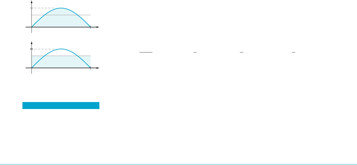
with the geometric interpretation of average value: If f is positive on [a, b], then the

area under the graph of f over [a, b] equals the area of the rectangle with base [a, b]

and height f

avg

f ðxÞdx ¼ f

avg

ðb 2 aÞ:

This is illustrated in Figure 2.

⁄ EX

AMPLE 10 Compute the average value of f (x) 5 sin(x)

for 0 # x # π.

Solution Because 2 cos( x )

is an antiderivative of sin(x), we use Theorem 3 from

Section 5.2 to calculate the average value of f on [0, π] as follow s:

avg

π 2 0

sinðxÞdx 5





2cosðxÞ







2ð21Þ2 ð21Þ



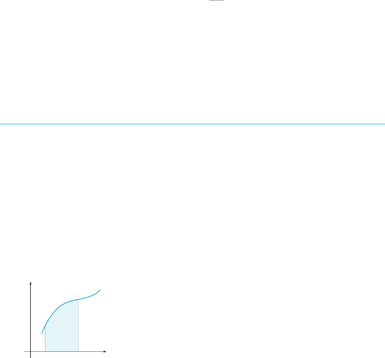
See Figure 3. Notice that the average value is not the

average of the values of f at

the endpoints (which is 0 in this case). It is not the average of the maximum and

minimum values of f on the interval (which is 1/2 in this case). Also, it is not the

value of f at the midpoint of the interval (which is 1 in this case).

QUICK QUIZ

1. What is

tan

ðxÞdx

2. Calcul ate

dx:

3. If

f ðxÞdx 5 3and

f ðxÞdx 525, then what is

3 f ðxÞ dx?

4. What is the average value of f (t) 5 t

for 1 # t # 4?

Answers

1. 0 2. 218

3. 24 4. 7

ave

y  sin(x)

y  2

m Figure 3 The shaded regions

have equal areas.

EXERCISES

Problems for Practice

1. Suppose that

f ðxÞdx 528 and

f ðxÞdx 5 12. Evalu-

ate

f ðxÞdx.

2. Suppose that

gðxÞdx 526 and

gðxÞdx 5212.

Evaluate

gðxÞdx.

3. Suppose that

f ðxÞdx 527 and

gðxÞdx 524.

Evaluate

ð4f ðxÞ2 9gðxÞÞdx.

4. Suppose that

f ðxÞdx 5 6. Evaluate

f ðxÞdx.

5. Suppose that

f ðxÞdx 5 6 and

f ðxÞdx 524. Evalu-

ate

f ðxÞdx.

6. Suppose that

gðxÞdx 5 5 and

gðxÞdx 5 12. Eval-

uate

gðxÞdx.

7. Suppose that

f ðxÞdx 5 5 and

gðxÞdx 5 15. Evaluate

ð6f ðxÞ2 7gðxÞÞdx.

8. Suppose that

f ðxÞdx 5 2. Evaluate

24f ðxÞ dx.

9. Suppose that

ð23f ðxÞ =4Þ dx 5 7. Evaluate

ð6f ðxÞ1 1Þdx.

10. Suppose that

f ðxÞdx 5 5. Evaluate

ð3f ðxÞ2 5xÞdx.

11. Suppose that

f ðxÞ=3dx 5 2. Evaluate

3f ðxÞdx.

12. Suppose that



2f ðxÞ2 x



dx 5 6. Evaluate

f ðxÞdx.

13. Suppose that

f ðxÞdx 5 0 and

gðxÞdx 5 0. Evaluate

ðf ðxÞ2 3gðxÞ1 5Þdx.

14. Suppose that

ð3f ðxÞ2 xÞdx 5 6 and

ð2x 1 4gðxÞÞdx 528. Evaluate

ðf ðxÞ2 5gðxÞÞdx.

c In Exercises 15220, compute the average value f

avg

of f

over [a, b] and ﬁnd a point c in (a, b) for which f (c) 5 f

avg

Illustrate the geometric signiﬁcance of c with a sketch

accompanied by a description. b

15. f (x) 5 1 1 xa5 1, b 5 5

406 Chapter 5 The Integral

16. f (x) 5 x

a 5 0, b 5 2

17. f ðxÞ5

ﬃﬃﬃ

a 5 1; b 5 4

18. f (x) 5 1/x

a 5 1/2, b 5 2

19. f (x) 5 12x

1 5 a 5 0, b 5 3

20. f (x) 5 2x 1 2/xa5 1, b 5 e

c In Exercises 21228, compute the average value of f over

[a, b] b

21. f (x) 5 8 2 x

a 524, b 5 2

22. f (x) 5 x

1 1/x

a 5 1, b 5 3

23. f ðxÞ5

ﬃﬃﬃ

2 1=

ﬃﬃﬃ

a 5 1; b 5 4

24. f (x) 5 e

a 5 0, b 5 2

25. f (x) 5 cos(x) a 5 0, b 5 π/2

26. f (x) 5 sin(x) a 52π/2, b 5 π/3

27. f (x) 5 sec

(x) a 5 0, b 5 π/4

28. f (x) 5 sec(x) tan(x) a 5 π/4, b 5 π/3

c In each of Exercises 29232, an integral is given. Do not

attempt

to calculate its value V. Instead, use the inequalities

of line (5.3.5) (as in Example 8) to ﬁnd numbers A and B such

that A # V # B. b

29.

ﬃﬃﬃﬃﬃﬃﬃﬃﬃﬃﬃﬃﬃ

9 1 x

30.

ﬃﬃﬃﬃﬃﬃﬃﬃﬃﬃﬃ

3 1 x

31.

ð25 2 x

21=2

32.

π=3

π=4

sin

ðxÞdx

Further Theory and Practice

c In Exercises 33236, use the information to determine

f ðxÞdx and

gðxÞdx. b

33.

ðf ðxÞ2 3gðxÞÞdx 5 3;

ð26gðxÞ1 9f ðxÞÞdx 5 6

34.

ðf ðxÞ1 4gðxÞÞdx 5 5;

3gðxÞdx 522

35.

ðf ðxÞ1 2gðxÞÞdx 527;

ðgðxÞ2 f ðxÞÞdx 5 4

36.

ðf ðxÞ2 7gðxÞÞdx 529;

ðgðxÞ1 f ðxÞÞdx 5 0

c In Exercises 37244, use Theorem 3 from Section 5.2 with

one

or more parts of Theorem 1 from this section to calculate

the given deﬁnite integral. b

37.

3x 2 5

38.

xð4x

2 2Þ dx

39.

ð6x

1 e

Þdx

40.

ðx 2 2Þðx 1 3Þ dx

41.

ﬃﬃﬃ

ð1 2 xÞdx

42.

1=4

x 2 1

ﬃﬃﬃ

2 1

43.

ð2 2 e

Þdx

44.

π=2

π=4

xsinðxÞ1 1

45. Suppose that p and q are constants with p . 0 and q . 0.

Is it ever true that

 x

dx 5

dx 

dx?

46. When is it true that

f ðxÞ1dx 5

f ðxÞdx 

1 dx?

47. Find an example of a function f, a function g, and values

of a and b such that

f ðxÞ

gðxÞ

dx 6¼

f ðxÞdx

gðxÞdx

c In each of Exercises 48251, a deﬁnite integral is given. Do

not

attempt to calculate its value V. Instead, ﬁnd the extreme

values of the integrand on the interval of integration, and use

these extreme values together with the inequalities of line

(5.3.5) to obtain numbers A and B such that A # V # B. b

48.

1 5

x 1 2

49.

2 4x 1 5

50.

ðx 1 1Þ

1 1

51.

2x=2

52. Use trigonometric identities to evaluate

π=2

cos

ðx=2Þdx

and

sin

ðxÞdx.

c In each of Exercises 53258, F (x)

is a function of a variable

x that appears in a limit (or in the limits) of integration of a

given deﬁnite integral. Express F (x) explicitly by calculating

the integral. b

53. FðxÞ5

ð3t

1 1Þdt

54. FðxÞ5

π=6

2 cosðtÞdt

55. FðxÞ5

ð2t 1 1=t

Þdt

56. FðxÞ5

ð2t 1 3t

Þdt

57. FðxÞ5

ﬃﬃ

58. FðxÞ5

ð2 1

ﬃﬃ

Þdt

c In each of Exercises 59262, verify that inequality (5.3.6)

holds

for the given integrand f and interval I of integration. b

59. f (x) 5 πx 2 3 I 5 [0,

60. f (x) 5 sin(x) 2 cos(x) I 5 [0, π/3]

61. f (x) 5 1 2 9x

I 5 [22, 1]

62. f (x) 5 e

2 7 I 5 [0, 2]

63. Let P

(x) 5 (3x

2 1)/2. This polynomial is called the

degree 2 Legendre polynomial. Show that if Q (x) 5

Bx 1 C for constants B and C, then

5.3 Rules for Integration 407

ðxÞQðxÞdx 5 0:

64. Let P

(x) 5 (5x

2 3x)/2. This polynomial is called the

degree 3 Legendre polynomial. Show that if Q (x) 5

1 Bx 1 C for constants A, B, and C, then

ðxÞQðxÞdx 5 0:

Calculator/Computer Exercises

c In each of Exercises 65268, a deﬁnite integral is given. Do

not attempt to calculate its value V. Instead, ﬁnd the extreme

values of the integrand on the interval of integration, and use

these extreme values together with the inequalities of line

(5.3.5) to obtain numbers A and B such that A # V # B. b

65.

1 1 x

66.

3=2

ﬃﬃﬃ

2 sinð xÞÞ dx

67.

π=2

ð3 sinðx

Þ1 cosðxÞÞ dx

68.

1=2

lnð1 1 xÞ dx

c In Exercises 69272, compute the average value f

avg

of f

over [a, b], and ﬁnd a value of c in (a, b) at which f attains this

average value. Illustrate the geometric meaning of the Mean

Value Theorem for Integrals with a graph. b

69. f (x) 5 x 1 sin

(x) a 5 0, b 5 π/2

70. f (x) 5 x

1 cos (x) a 5 0, b 5 π

71. f (x) 5 x

1 4/xa5 2 b 5 6

72. f (x) 5 (x

2 4x 1 6)/3 a 5 0, b 5 2

5.4 The Fundamental Theorem of Calculus

Theorem 3 from Section 5.2 tells us that, if f is continuous on [a, b]andif f has an

antiderivative F on [ a , b], then

f ðtÞdt 5 FðbÞ2 FðaÞ: ð5:4:1Þ

This equation is the ﬁrst part of the Fundamental Theorem of Calculus. In this

section, we learn that every continuous function f has an antiderivative. This fact

constitutes the second part of the Fundamental Theorem of Calculus.

In the analytic proof of the second part of the Fundamental Theorem of

Calculus, we assume only that f is a continuous function. However, we will motivate

this theorem geometrically by considering areas. Therefore for the purposes of this

discussion, we suppose that f is positive in addition to being continuous. To this

function f we associate an area function F that is deﬁned by

FðxÞ5

f ðtÞdt: ð5:4:2Þ

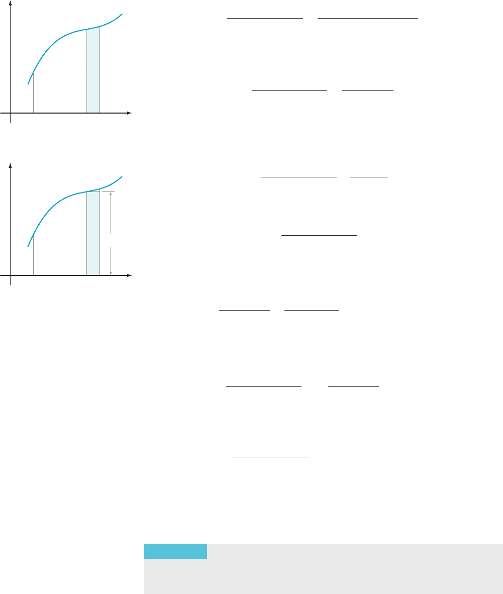
Figure 1 shows the graph of y 5 f (t) in the ty-plane. As Figure 1 indicates, the value

of F (x) is the area of the region that lies below the graph of f, above the t-axis, and

between the vertical lines t 5 a and t 5 x. Notice that F is a function of the upper

limit x of integration, not of the symbol t that appears within the integral. Also, we

do not assume that an explicit formula for F (x) can be found. It is known, for

example, that the area function FðxÞ5



2 1 cos ðt



dt cannot be expressed in

terms of ﬁnitely many elementary functions. It is precisely such area functions that

we wish to understand.

The main result of this section is that F is an antiderivative of f. In other words,

F is a differentiable function and F

5 f. To prove these assertions, we refer to the

deﬁnition of the derivative and look at the difference quotient:

y  f(t)

Area  F(x)

m Figure 1

408 Chapter

5 The Integral

Fðx 1 ΔxÞ2 FðxÞ

Δx

x1Δx

f ðtÞdt 2

f ðtÞdt

Δx

We now use Theorem 3 from Section 5.3 to rewrite the numerator of the right

side of this equation. We obtain

Fðx 1 Δ x Þ2 FðxÞ

Δx

x1Δx

f ðtÞdt

Δx

: ð5:4:3Þ

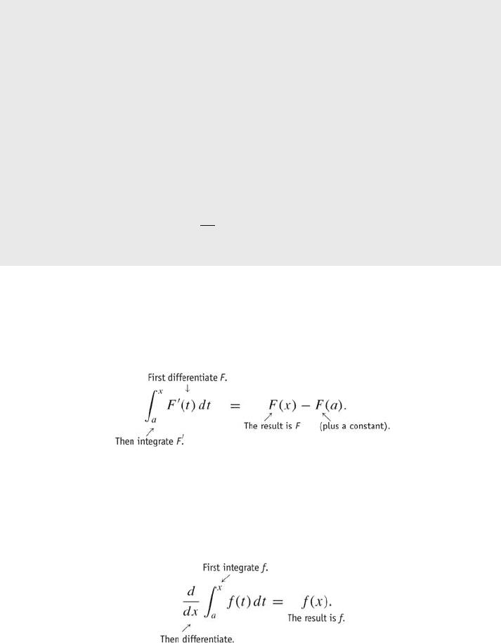
The numerator

x1Δx

f ðtÞdt represents the area of the shaded region in Figure 2.

When Δx is small, the integral

x1Δx

f ðtÞdt is nearly equal to the area of a rectangle of

base Δx and height f (x)(seeFigure3).Therefore

Fðx 1 Δ x Þ2 FðxÞ

Δx



f ðxÞΔx

Δx

as Δx - 0. Thus we have intuitively deduced that

lim

Δx-0

Fðx 1 Δx Þ2 FðxÞ

Δx

5 f ðxÞ:

We can make this argument rigorous by appealing to the Mean Value Theorem for

Integrals, which tells us that there exists a c between x and x 1 Δx such that

x1Δx

f ðtÞdt

Δx

ðx 1 Δ x Þ2 x

x1Δx

f ðtÞdt 5 f ðcÞ: ð5:4:4Þ

By combining equations (5.4.3) and (5.4.4), we ﬁnd that for any Δx,thereisac

between x and x 1 Δx such that

Fðx 1 Δ x Þ2 FðxÞ

Δx

ð5:4:3Þ

x1Δx

f ðtÞdt

Δx

ð5:4:4Þ

f ðcÞ: ð5:4:5Þ

Because c lies between x and x 1 Δx, it follows that c - x as Δx - 0. From these

observations, we obtain

lim

Δx-0

Fðx 1 Δ x Þ2 FðxÞ

Δx

5 lim

Δx-0

f ðcÞ5 lim

c-x

f ðcÞ5 f ðxÞ;

where the last equality results from the continuity of f. This equation means that the

derivative of F at x exists and equals f (x). In short, F is an antiderivative for f.The

theorem that follows combines the two parts of the Fundamental Theorem of

Calculus.

THEOREM 1

(Fundamental Theorem of Calculus). Let f be a continuous

function on the interval [a, b].

a. If F is any antiderivative of f on [a, b], then

x  xax

y  f(t)

F(x)

m Figure 2 Area 5

x1Δ

f (t) dt

f(x)

x  xax

y  f(t)

F(x)

m Figure 3

x1Δ

f (t) dt is ap-

proximately the area f (x) Δx of

the shaded rectangle.

5.4 The Fundamental Theorem of Calculus 409

f ðtÞdt 5 FðbÞ2 FðaÞ:

b. The function F deﬁned by

FðxÞ5

f ðtÞdt ða # x # bÞ

is an antiderivative of f. This function F is continuous on [a, b] and

ðxÞ5 f ðxÞða , x , bÞ:

In Leibniz notation,

f ðtÞdt 5 f ðxÞ: ð5:4:6Þ

Together, the two parts of the Fundamental Theorem inform us that differ-

entiation and integration are inverse operat ions. Let us apply the ﬁrst part of the

Fundamental Theorem to a continuous derivative F

. Because F is an anti-

derivative of F

, we obtain

Thus if we differentiate F and integrate the derivative, then we recover the function

F with which we started (plus the constant 2F (a)). The second part of the Fun-

damental Theorem, equation (5.4.6) , tells us that if we integrate the function f and

then differentiate with respect to the upper limit of integration, then we recover the

function f with which we started:

We therefore think of integration and differentiation as processes that are inverse

to one another.

Examples Illustrating

the First Part of the

Fundamental Theorem

We have been using the ﬁrst part of the Fundamental Theorem of Calculus since

Section 5.2. The integrands in the examples we now consider require greater care

than those found in previous sections.

⁄ EX

AMPLE 1 Compute

dt:

Solution To

use the ﬁrst part of the Fundamental Theorem, we need to ﬁnd an

antiderivative for the function f (t) 5 e

. Notice that

410 Chapter 5 The Integral

5 2e

; or





5 e

Therefore FðtÞ5

is a suitable antiderivative, and

dt 5 FðtÞ



t5 1

t5 0

ðe

2 1Þ: ¥

INSIGHT

Remember that a deﬁnite integral represents a deﬁnite number or

expression. Including an arbitrary constant of integration in the ﬁnal answer (as we would

for an indeﬁnite integral) is wrong. In Example 1, we used the Fundamental Theorem of

Calculus to compute the deﬁnite integral

f ðtÞdt . Accordingly, we ﬁrst computed the

indeﬁnite integral (or antiderivative)

f ðtÞdt . At this stage, had we added a constant C to

the indeﬁnite integral F (t) 5 e

/2, it would not have mattered:

dt 5



1 C





t5 1

t5 0



1 C





1 C





1 C





2 C



ðe

2 1Þ:

The constant C cancels out and does not appear in the ﬁnal answer. The deﬁnite integral

dt represents a unique number. The only correct answer is (e

2 1)/2. In particular,

the answer “(e

2 1)/2 1 C where C is an arbitrary constant” is incorrect.

⁄ EXAMPLE 2 Calculate

sin

ðtÞdt:

Solution Becau

se it is not immediately clear what an antiderivative for sin

(t)

might be, we ﬁrst rewrite the integrand using the Half-Angle Formula (equation

(1.14) from Section 1.6 in Chapter 1),

sin





1 2 cosðθÞ

Setting θ 5 2t, we obtain sin

(t) 5 (1 2 cos(2t))/2. We substitute this identity into

our original integral and ﬁnd the required antiderivative:

sin

ðtÞ dt 5

ð1 2 cosð2tÞÞdt 5



t 2

sinð2tÞ





t5π

t50

: ¥

INSIGHT

The Solution to Example 2 begins with the remark that ﬁnding an anti-

derivative of sin

(t) is not obvious. A common error is to think that because t

/3 is

an antiderivative of t

, it must follow that sin

(t)/3 is an antiderivative of sin

(t). This

reasoning is incorrect. We must use the Chain Rule when we differentiate sin

(t)/3. We

obtain



 sin

ðtÞ



 3 sin

ðtÞ

sinðtÞ5 sin

ðtÞcosðtÞ;

which shows that sin

(t)/3 is an antiderivative of sin

(t) cos(t), not of the given integrand

sin

( t).

5.4 The Fundamental Theorem of Calculus 411

Examples of the

Second Part of the

Fundamental Theorem

In the second part of the Fundamental Theorem, we deﬁne a function in terms of

an integ ral. It is important that you understand this part because it will be the key

to many applications of the integral and also the key to our rigorous approach to

the logarithm funct ion in the next section.

⁄ EX

AMPLE 3 The hydrostatic pressure exerted against the side of a certain

swimming pool at depth x is

PðxÞ5

t ðsinð2tÞ1 1Þdt:

What is the rate of change of P with respect to depth when the depth is 4?

Solution We

have not yet learned how to calculate an antiderivative of f (t) 5

t (sin(2t) 1 1). However, the second part of the Fundamental Theorem tells us that

we do not need to evaluate the integral that deﬁnes P(x) in order to compute P

(x).

Because P (x) 5

f ðtÞdt; Theorem 1b tells us that

ðxÞ5 f ðxÞ5 x ðsinð2xÞ1 1Þ:

In particular, P

(4) 5 4 (sin(8) 1 1) 7.957. ¥

⁄ EXAMPLE 4 Calculate the derivative of FðxÞ5

sinð

ﬃﬃ

Þdt with respect

to x.

Solution The

Fundamental Theorem tells us how to different iate an integral with

respect to its upper limit of integration. This exampl e involves an upper limit that is

a function of the variable of differentiation. We must use the Chain Rule. If we let

u 5 x

, then

FðxÞ¼

sinð

ﬃﬃ

Þdt ¼

sin



ﬃﬃ







¼ sinð

ﬃﬃﬃ

Þ2x

¼ sinð

ﬃﬃﬃﬃﬃ

Þ2x ¼ 2x sinðjxjÞ: ¥

Example 4 illustrates an extension of formula (5.4.6). If u is

a function of x,then

uðxÞ

f ðtÞdt 5 f ðuðxÞÞ 

uðxÞ: ð5:4:7Þ

⁄ EX

AMPLE 5 Calculate the derivative of FðxÞ5

expð2t

Þdt with

respect to x.

Solution The

Fundamental Theorem tells us how to different iate an integral with

respect to its upper limit of integration, but in this example, the variable of

differentiation is the lower limit of integration. There is a simple remedy: We

reverse the order of integration. Thus

expð2 t

Þdt 52

expð2t

Þdt 52expð2x

Þ: ¥

Example 5 illustrates another extension of formula (5.4.6). We can combine the

ideas

of Examples 4 and 5 to state the extension as follows:

uðxÞ

f ðtÞdt 52f ðuðxÞÞ

uðxÞ: ð5:4:8Þ

412 Chapter 5 The Integral

⁄ EXAMPLE 6 Let F be deﬁned by FðxÞ5

sinðxÞ

cosðxÞ

ﬃﬃﬃﬃﬃﬃﬃﬃﬃﬃﬃﬃ

1 2 t

dt for 0, , x , π/2.

Differentiate F(x) with respect to x.

Solution This

example involves both upper and lower limits of integration that

depend on x. None of the formulas (5.4.6), (5.4.7), and (5.4.8) is immediately

applicable. However, if we choose any ﬁxed number a and, using (5.3.1), write

FðxÞ 5

sinðxÞ

cosðxÞ

ﬃﬃﬃﬃﬃﬃﬃﬃﬃﬃﬃﬃ

1 2 t

dt 5

cosðxÞ

ﬃﬃﬃﬃﬃﬃﬃﬃﬃﬃﬃﬃ

1 2 t

dt 1

sinðxÞ

ﬃﬃﬃﬃﬃﬃﬃﬃﬃﬃﬃﬃ

1 2 t

sinðxÞ

ﬃﬃﬃﬃﬃﬃﬃﬃﬃﬃﬃﬃ

1 2 t

dt 2

cosðxÞ

ﬃﬃﬃﬃﬃﬃﬃﬃﬃﬃﬃﬃ

1 2 t

dt;

then we can differentiate each of the two summands using formula (5.4.7):

FðxÞ 5

ﬃﬃﬃﬃﬃﬃﬃﬃﬃﬃﬃﬃﬃﬃﬃﬃﬃﬃﬃﬃﬃﬃ

1 2 sin

ðxÞ

sinðxÞ2

ﬃﬃﬃﬃﬃﬃﬃﬃﬃﬃﬃﬃﬃﬃﬃﬃﬃﬃﬃﬃﬃﬃﬃ

1 2 cos

ðxÞ

cosðxÞ

ﬃﬃﬃﬃﬃﬃﬃﬃﬃﬃﬃﬃﬃﬃﬃ

cos

ðxÞ

cosðxÞ2

ﬃﬃﬃﬃﬃﬃﬃﬃﬃﬃﬃﬃﬃﬃ

sin

ðxÞ

ð2sinðxÞÞ

5 jcosðxÞjcosðxÞ1 jsinðxÞjsinð x Þ

5 cos

ðxÞ1 sin

ðxÞ because 0 , x , π=2

5 1: ¥

INSIGHT

In Chapter 6, we learn how to directly calculate the integral that deﬁnes the

function F from Example 6. But, as with Examples 3, 4, and 5, it is not necessary to

compute F to obtain F

. It is therefore interesting to observe that our calculation F

(x) 1

actually gives us an indirect way to calculate F(x). Because G (x) 5 x is also an anti-

derivative of the constant function 1, Theorem 5 from Section 4.1 of Chapter 4 tells us that

F (x) 5 G (x) 1 C 5 x 1 C for some constant C. Substituting x 5 0 into this last equation,

we obtain

C 5 Fð0Þ5

sinð0Þ

cosð0Þ

ﬃﬃﬃﬃﬃﬃﬃﬃﬃﬃﬃﬃ

1 2 t

dt 52

ﬃﬃﬃﬃﬃﬃﬃﬃﬃﬃﬃﬃ

1 2 t

|ﬄﬄﬄﬄﬄﬄﬄﬄﬄﬄﬄﬄ{zﬄﬄﬄﬄﬄﬄﬄﬄﬄﬄﬄﬄ}

Area of 1=4-unit circle

ðsee Figure 4Þ

Therefore F (x) 5 x 2 π /4.

QUICK QUIZ

1. Suppose that FðxÞ5

sinðt

Þdt. What is F

(2)?

2. Suppose that FðxÞ5

ð1 1 t

dt. What is F

(2)?

3. Suppose that FðxÞ5

2 1 t

1 1 t

dt: What is F

(1)?

4. Evaluate

ðxe

Þdx:

Answers

1. sin(4) 2. 21/5

3. 7/6 4. e

Arc of

unit circle

Area  p

1  t

y 



m Figure 4

5.4 The Fundamental Theorem of Calculus 413

EXERCISES

Problems for Practice

c Use the ﬁrst part of the Fundamental Theorem of Calculus

together with the ideas of Examples 1 and 2 to evaluate the

deﬁnite integrals in Exercises 1210. b

π=4

π=6

12cosð2xÞdx

sinðx=2Þdx

π=2

2π=3

4sinð2xÞdx

π=2

2π=4

cos

ðxÞdx

π=2

secðx=3Þtanðx=3Þdx

π=8

2π=8

sec

ð2xÞdx

π=4

sin

ð2xÞdx

10.

π=4

2π=4

cos

ð4xÞdx

c In Exercises 11220, calculate FðxÞ5

f ðtÞdt: b

11. f ðtÞ5 3t

1 1 a 521

12. f ðtÞ5 sinðt Þ a 5 π=4

13. f ðtÞ5 4t

1=3

a 5 8

14. f ðtÞ5 e

a 521

15. f ðtÞ5 ðe

1 e

Þ=2 a 5 0

16. f ðtÞ5 sec

ðtÞ a 5 0 ð2π=2 , x , π=2Þ

17. f ðtÞ5 secðtÞtanðtÞ a 52π=4 ð2π=2 , x , π=2Þ

18. f ðtÞ5 1=ta5 e ð0 , xÞ

19. f ðtÞ5 15

ﬃﬃ

ð1 1 tÞ a 5 1 ð0 , xÞ

20. f ðtÞ5 ð3t 1 1=2Þ=

ﬃﬃ

a 5 4 ð0 , xÞ

c In each of Exercises 21228, calculate the derivative of

F (x)

with respect to x. b

21. FðxÞ5

ð2t 1 1Þðt 1 2Þdt

22. FðxÞ5

1=3

ﬃﬃ

1 3Þdt

23. FðxÞ¼

þ 2t

þ 3t þ 6

t þ 2

24. FðxÞ5

tan

ðtÞdt

25. FðxÞ5

tanðt

Þdt

26. FðxÞ5

sinðt

Þdt

27. FðxÞ5

ﬃﬃﬃﬃﬃﬃﬃﬃﬃﬃ

1 1 t

28. FðxÞ5

lnðtÞdt

c In each of Exercises 29234, calculate the derivative of

F (x)

with respect to x. b

29. FðxÞ5

π=4

cosð4tÞdt

30. FðxÞ5

π=4

ﬃﬃﬃﬃﬃﬃﬃﬃﬃﬃﬃﬃﬃﬃﬃﬃﬃﬃﬃﬃ

1 1 cosðtÞ

31. FðxÞ5

π=4

cotðtÞdt

32. FðxÞ5

ﬃﬃﬃﬃﬃﬃﬃﬃﬃﬃﬃﬃﬃﬃ

2 1

33. FðxÞ5

ﬃﬃﬃﬃﬃﬃﬃﬃﬃﬃﬃﬃﬃﬃﬃﬃﬃﬃﬃﬃﬃ

2 2 sin

ðtÞ

34. FðxÞ5

cosð

ﬃﬃ

Þdt

c In each of Exercises 35242, follow the method of Example

to calculate F

(x). b

35. FðxÞ5

sinð2tÞdt

36. FðxÞ5

ﬃﬃﬃﬃﬃﬃﬃﬃﬃﬃ

1 1 t

37. FðxÞ5

cotðtÞdt

38. FðxÞ5

ﬃﬃ

ð1 1 t

21=2

39. FðxÞ5

exp ðxÞ

exp ð2xÞ

lnðtÞdt

40. FðxÞ5

cos ðt

Þdt

41. FðxÞ5

ﬃﬃ

ﬃﬃﬃﬃﬃﬃﬃﬃﬃﬃﬃﬃﬃﬃ

2 1

42. FðxÞ5

ﬃﬃﬃﬃﬃﬃﬃﬃﬃﬃﬃﬃ

1 1 t

Further Theory and Practice

c In Exercises 43246, compute F

and F

. Determine the

intervals on which F is increasing, decreasing, concave up,

and concave down. b

43. FðxÞ5

tðt 2 1Þdt

44. FðxÞ5

t expð2 tÞdt

45. FðxÞ5

t lnðtÞdt 0 , x

46. FðxÞ5

ﬃﬃﬃﬃﬃﬃﬃﬃﬃﬃﬃﬃ

1 1 t

2 tÞdt

47. Suppose that f is continuous on (2a, a) and that f is an

odd function: f (2t) 52f (t). For x in (2a, a), let

Fð xÞ5

f ðtÞdt. Show that F

5 0, and use this result to

evaluate F.

48. Suppose that f is continuous on (2a, a)andthatf is an even

function: f (2t) 5 f (t). Differentiate FðxÞ5

f ðtÞdt 2

f ðtÞdt with respect to x, and use your result to show that

f ðtÞdt 5

f ðtÞdt.

49. Suppose a body travels in a line with position p (t) at time

t and velocity v (t) at time t. Show that

vðtÞdt 5 pðbÞ2 pðaÞ:

c In Exercises 50253, verify that point P is

on the graph

of function F, and calculate the tangent line to the graph of

F at P. b

50. FðxÞ5

ﬃﬃ

dt P 5 ð4; 28Þ

51. FðxÞ5

1=tdt P5 ðe; 1Þ

52. FðxÞ5

dt P 5 ð7; 93Þ

53. FðxÞ5

cosðtÞdt P 5 ðπ=6; 1=2Þ

414 Chapter 5 The Integral