Canete J.F. System Engineering and Automation: An Interactive Educational Approach

Подождите немного. Документ загружается.

108

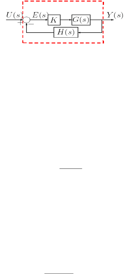
Fig. 4.17 Close-loop config

poles of the system can be c

This is actually a typ

controlled, H(s) represen

is a gain that amplifies th

happens, it means that

therefore, no actuation is

Chapter 5 goes in det

are going to cope with

parameter K. This behav

of poles, and the root loc

Recalling Chapter 3

configuration of fig. 4.17

being the characteristic e

In this equation the para

roots, and therefore the p

Example 4.8

Considering

Obtain the close-loop tra

different values of K.

Solution

The close-loop transfer f

4 System Response Analy

ration. Through the root locus, all the possible locations of t

lculated in function of the parameter K.

cal proportional control where G(s) is the plant to

s a sensorial system that measures the plan outpu

, and

error signal given to G(s). When error is zero, in case

(s)=U(s), and the input to the system G(s) is also zer

arried out.

il on proportional and other control systems, by now

he behavior of the close-loop system according to t

or, as commented before, will be defined by the positi

s technique comes to depict their possible locations.

the equivalent transfer function of the close-lo

is:

(4.3

uation

eter K, and thus, variations in its value will modify

sition of the poles.

nsfer function and the position of its poles according

nction is:

()

tot

KGH

() () 1

710

sHs

1()()0KG s H s+=

)

4.3 Root Locus 109

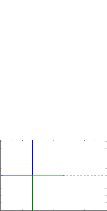
Giving values to the gain K and calculating the roots of the characteristic equation

for this second-order system, we obtain

K P1 P2

0 -5 -2

1 -4.62 -2.38

2 -4 -3

2.25 -3.5 -3.5

3 -3.5+0.872i -3.5-0.872i

6.5 -3.5+2.06i -3.5-2.06i

From this we can deduce that if 0

≤ K ≤ 2.25 the system is overdamped, that is it

has different and real poles, for K=2.25 the system is critically damped, i.e. it has

two real and equal poles, finally if K

≥ 2.25, the system is underdamped,

exhibiting a oscillating behavior due to the presence on complex conjugated poles.

If we depict the position of the poles as long as the value of K is increasing we

obtain:

Fig. 4.18 Root Locus example. Illustration of how the poles move as long as the parameter

K increases.

That is, we can rapidly observe the position of each pole, and therefore

inference the behavior of the final system, in a plot like the one shown in

fig. 4.18. Obviously relying on a systematic calculation of the roots of the

characteristic equation to depict the possible position of the poles based on a given

parameter is not practical at all and a set of recipes are available for sketching it.

4.3.1 Root Locus Recipe

There exists a set of simple steps for sketching the root locus of a given system.

They are mathematically derived from the complex nature of the characteristic

()

710

ss K

+++

Root Locus

Real Axis

Imag Axis

-5 -4.5 -4 -3.5 -3 -2.5 -2 -1.5 -1 -0.5 0

-2.5

-2

-1.5

-1

-0.5

0.5

1.5

2.5

110 4 System Response Analysis

equation. That is, given expression (4.38), we can distinguish the real and complex

part of the equation and rewrite it as shown in (4.39).

(4.38)

(4.39)

That is,

(4.40)

(4.41)

Equation (4.40) is known as the magnitude condition and can be used to calculate

the value of the parameter K for a particular position of the poles. Equation (4.41)

is called the angle condition and permits us to determine whether a particular point

of the s-plane belongs or not to the root locus, i.e. if there exist a value for K for

which one of the poles of the system are located at that particular point.

These two equations are the basis for the root locus method.

Example 4.9

Check the application of the magnitude and angle conditions to the system

At the test point s, .

Solution

G(s)H(s) can be rewritten as:

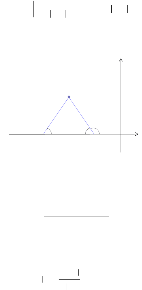
For the test point (see fig. 4.19), angle condition is computed as:

And therefore this condition holds for this test point. Actually it holds for

1()()0 ()()1KG s H s KG s H s+=⇒ =−

() () () () 1 0KG s H s KG s H s j∠=−+

() () 1KG s H s =

() () 1 (2 1), 0, 1, 2,...KG s H s k k

∠=∠−=+=±±

() () 1

710

Gs Hs

3.5sj=− +

() ()

(2)(5)

GsHs

[]

(2)(5) ( )

(2)(5)

πθ θ π

∠ =−∠ + −∠ + =− − + =−

3.5 , [0, )sxjx=− ± ∈ ∞

4.3 Root Locus 111

Now we have confirmed that s

=-3.5+j belongs to the root locus we want to figure

out the value of K that moves one of the poles to this position. For that we rely on

the magnitude condition:

Yielding the value of K=3.6, which confirms what we figure out by sequentially

solving the characteristic function for different values of K.

Fig. 4.19 Root Locus example where the point s=s

is being checked whether it belongs or

not to the root locus (more description in the text).

In general, for an n-order system, the characteristic equation is given by

being

(4.42)

and the magnitude and angle condition computed as:

(4.43)

(4.44)

1253.6

(2)(5) 2 5

Ks s

ss ss

==⇒ =+ +=

++ ++

-5

θθ

jω

-2

-2.25

+5| |s

+2|

∠

() 1Fs =−

( )( )...( )

()

( )( )...( )

Ks z s z s z

spsp sp

++ +

( ) ( ) ( ) (2 1), 0,1,2,...

Fs s z s p k k

∠=∠+−∠+= + =

∑∑

() 1

∏

112 4 System Response Analysis

Next, a list of steps are given based on these conditions for sketching the root

locus.

Step 1. Placement of the poles and zeroes of G(s)H(s) on the s-plane

Firstly it is recommendable to rewrite the equation

(4.45)

Mark on the s-plane the poles p

with a cross ‘x’ and the zeroes z

with a small

circle ‘o’. Note that when K=0, equation (4.45) is reduced to

(4.46)

And thus, the poles of the closed-loop system are identical to the poles in the

open-loop configuration, that is G(s)H(s). Also notice that as long as K tends to ∞,

the roots of the equation (4.45) coincides with the zeroes of G(s)H(s):

(4.47)

Thus, at this first step we obtain significant information about the root locus

sketch: Root locus starts at the poles of the open-loop system, i.e. the root locus

will be made of n strokes, each one starting at a pole of G(s)H(s), when K=0, and

some of them, precisely m, ending at the zeroes of G(s)H(s), when K

→∞.

Step 2. Root locus on the real axis

In this step we focus on which part of the real axis will be part of the root locus,

that is we are going to apply the angle condition to points s∈ℜ, and s=(-∞,∞). A

practical rule to remember tells us that “a given point s* lying on the real axis

belongs to the root locus if and only if the sum of the real poles and real zeroes

place on its right is an odd number”. This fanciful rule is based on the angle

condition and the need of yielding an odd multiple of π.

Example 4.10

Sketch the root locus over the real axis for the open-loop system

()

10()()0

()

KspKsz

+=⇒ ++ +=

∏

∏∏

∏

()0

sp+=

∏

11 1

()()0

lim ( ) ( ) ( )

nm m

ii i

sp sz

sp sz sz

→∞

++ +=

⎛⎞

++ + = +

⎜⎟

⎝⎠

∏∏

∏∏ ∏

4.3 Root Locus 113

Solution

After step 1, we locate the three poles at s=0, s=-1, and s=-2 as shown in fig. 4.20,

and test a point s between p

and p

, that is s∈(-2,-1). In absence of zeroes, the

angle condition is computed, in this example, as

Note that the presence of two poles on the right of s contributes with 2*

π, while

the pole on the left does not contribute. Thus, it is obvious that s is not a part of

the root locus, as well as any point in the interval (-2,-1). Following the same

argument, ∀s∈(-∞,-2] and ∀s∈[1,0], s is part of the root locus.

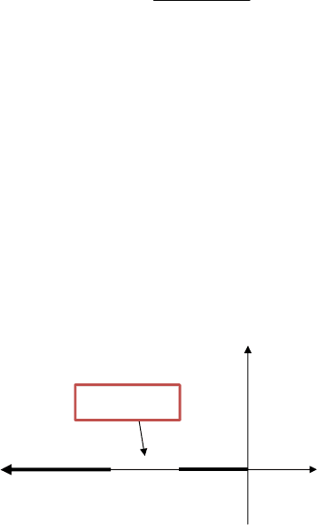
Fig. 4.20 Testing points on the real axis. Based on the angle condition, a point on the real

axis will belong to the root locus if the number of poles (and zeros) placed on its right is

odd. In this case, the s point does not belong to the root locus.

In this example, we observe that a certain direction is given to one segment of

the root locus to indicate the path followed by the pole p2 as long as the parameter

K increases. Thus, p2 tends to -∞ and it can be said that the root locus entails a

segment that starts at p2 and ends at -∞.

Step 3. Assessing asymptotes

In step 1 we stated that the segments of the root locus begins at the poles of

G(s)H(s) when K=0 and ends at the zeroes when K=∞. Normally, in causal

systems, the number of zeroes, m, is less than the number of poles, n, and thus

only m segments will end at a zero. The rest of segments, concretely m-n will tend

asymptotically to infinity. In the example of fig. 4.20, m=0 and n=3, i.e. there are

no zeroes, and thus the three segments that start at each pole asymptotically go

() ()

(1)(2)

GsHs

ss s

0 ( ) 0 2 (2 1), 0,1, 2,...

sp k k

ππ ππ

−∠+ =++= ≠ + =

∑

Punto de Prueba

p2 s

Test Point

114 4 System Response Analysis

forward to infinity. The angle of the asymptotes with respect the real axis can be

determined by the equation (4.48).

(4.48)

This expression comes from the application of the angle condition to a distant

point (ideally at the infinity). At that distant point the angles from poles and zeroes

can be assumed as equal and thus, they are cancelled, turning the angle condition

into

The place where the asymptotes cross the real axis is determined by the mass

center of the poles and zeroes as:

(4.49)

In the example of fig. 4.20 there are two asymptotes, with σ= ±

π/2, located at

=(-2-5)/2=-3.5.

Step 4. Identification of rupture points

In some occasions, two or more segments of the root locus collide at a particular

point of the s-plane, which is called a rupture point. That is, a rupture point occurs

when, given a certain value of K, the characteristic equation has roots with a

multiplicity greater than 1. Identifying these points will largely help to sketch the

root locus further away from the real axis.

Rupture points coincide with the maximum values of K so in practice, they are

computed by deriving K and solving the equation dK/ds=0. The solutions of this

equation, s*, fulfilling that K(s*)>0 are rupture points.

Example 4.11

Calculate the rupture points for the system

Solution

The characteristic function is:

(2 1)

0,1,2...

±+

−

() ()

−− −

−

∑∑

() () 1

710

Gs Hs

4.3 Root Locus 115

from which

And solving

Checking that it is really a maximum of the curve K, we have that

and thus s=-3.5 is a rupture point as revealed in the fig. 4.18.

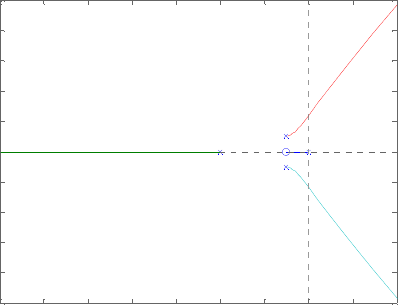
Although it is common to find rupture points lying on the real axis, there

are some cases where the roots of dK/ds are complex conjugates as illustrated in

fig. 4.21.

Fig. 4.21 Root Locus example for a system with 4 poles. It is made of four segments that

collides at three rupture points: s=-2 and s=-2±2.45j

Step 5. Determination of starting/ending angles

This step is a straightforward application of the angle condition. It provides us

with valuable information about the direction of the segments when starting at the

poles or when ending at the zeroes.

710 0ss K+++=

710 27

Ks s s

=− − − ⇒ =− −

0270 3.5

= ⇒ −−=⇒ =−

()

3.5 7( 3.5) 10 0K =− − − − − >

116 4 System Response Analysis

(4.50)

Step 6. Crossing points of the root locus with the complex axis

This is the last step for sketching a root locus and it is intimately related to

stability. In fact, in this step we calculate the value of the parameter K that made

unstable the close-loop system. At the moment, at least one pole of the close-loop

system will be located at the complex axis.

This step is not always applicable since there are cases where the system is

always stable regardless of the value of K

, as it is the example of fig. 4.18.

Example 4.12

Sketch the root locus for the system

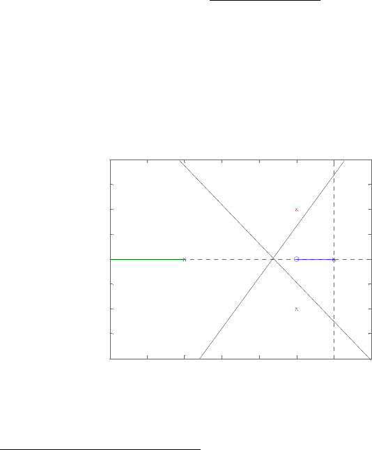
Solution

This system has one zero at s=-1 and four poles at s=0, s=-4 and s=-1±j.

The initial sketch is shown in fig. 4.22 where two segments lay on the real axis,

from s=-4 to infinity and from s=0 to s=-1and three asymptotes (n-m=3) with

Fig. 4.22 Root Locus example where two segments (those over the real axis) has been

traced. The asymptotes indicate the direction followed by the other two segments, starting

at the complex poles.

When K defined in the range [0,infinity).

pole poles zeroes

rest rest

zero zeroes poles

rest rest

ϕπϕ ϕ

=− +

∑

∑∑

() ()

(4)( 22)

GsHs

ss s s

+++

-6 -5 -4 -3 -2 -1 0 1

-2

-1.5

-1

-0.5

0.5

1.5

Root Locus

Real Axis

Imaginary Axis

4.3 Root Locus 117

angles 60,180 and 300°, crossing the real axis at σ

=-5/3. At this moment we realize

that there should be two segments more, starting at s=-1±j and that they have to tend

to infinity following the asymptotes, but how? Calculating the starting angle from

these poles we obtain ±26.6°, giving us a cue about their orientation.

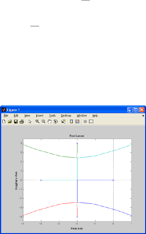
The sketch of the root locus is finished when the stability of the system and the

value of K and the location of the poles at the limit of the stability is computed. In

this example the Routh criteria yields that the system is unstable when K>24.78.

For this precise value, the characteristic equation has two roots at s=0±2.33j.

Therefore the root locus crosses the complex axis at ±2.33j. fig. 4.23 depicts the

root locus computed by the Matlab command

rlocus that confirms our initial

sketch was correct.

Fig. 4.23 Root Locus example depicted by rlocus. Note that there is a value of K that brings

the poles of the system to the right part of the s-plane, and thus, makes the system unstable.

In the following section the effect of adding/removing poles zeroes to the open-

loop system is commented.

4.3.2 Effects of Adding Poles/Zeros

Sometimes we are interested in modifying the behavior of a close-loop system to

obtain a particular response, e.g. reducing the overshoot, or to gain in stability.

One simple manner to do this is to add/remove poles/zeroes from the initial

configuration up to achieving our goal. In this section we analyze the effect of this

operation in the root locus.

Let’s begin with the simplest root locus, the root locus of a first-order system.

fig. 4.24 shows the root locus for a system with a pole at s=-5 and the close-loop

response for different values of K. Notice that as long as K increases, the pole

moves over the negative part of the real axis at the same time that the output

reduces the permanent error.

Root Locus

Real Axis

Imaginary Axis

-14 -12 -10 -8 -6 -4 -2 0 2 4

-10

-8

-6

-4

-2