Canete J.F. System Engineering and Automation: An Interactive Educational Approach

Подождите немного. Документ загружается.

98 4 System Response Analysis

Solution

The residues are:

>> [r,p]=residue(5,conv([1 0],[1 4 13]))

r =

-0.1923 + 0.1282i

-0.1923 - 0.1282i

0.3846

p =

-2.0000 + 3.0000i

-2.0000 - 3.0000i

That is,K

=0.3846, K

=-0.1923+0.1282j, and K

=-0.1923-0.1282j. Therefore,

K*2=-0.3846 and K*3=-0.257. With these values the response function is

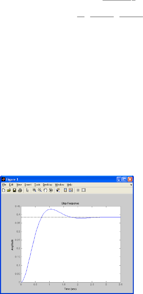
(see fig. 4.9 for a graphical representation):

>> G=5/(s^2+4*s+13)

Transfer function:

--------------

s^2 + 4 s + 13

>> step(G)

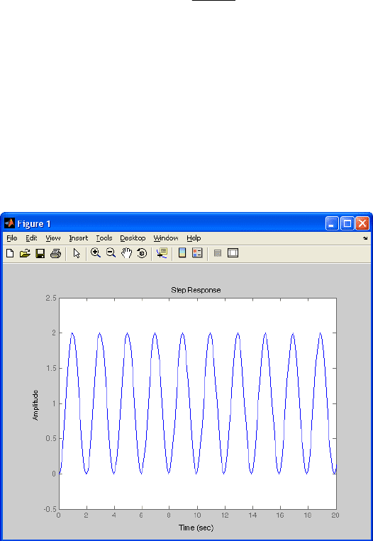
Fig. 4.9 Second-order system response with two complex conjugate poles. In contrast to

previous cases, when the system has complex poles, the response presents a sinusoidal behavior.

312

() ()

413

()

23 23

Ys Gs

sss

ss js j

=+ +

++ +−

()

( ) 0.3846 0.3846 cos(3 ) 0.257 (3 ) ( )

yt e t e sen t u t

−−

=− −

4.2 System Transient Response 99

Notice that in this case we have two parameters with influence in the response.

On the one hand, as commented, the magnitude of the poles (the real part) is

directly related to the time needed to achieve the steady-state, i.e. the final value.

On the other hand, the complex part of poles (which can be considered as zero for

the two first cases) is responsible for the frequency of the oscillations.

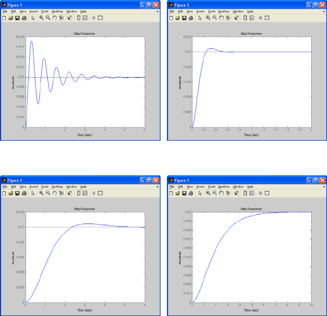
Fig. 4.10 illustrates the interrelation of both parameters studying the response

of a second-order system against unitary input step.

Poles at 1±10j

Poles at 10±10j

Poles at 1±1j

Poles at 1 (double poles)

Fig. 4.10 Contribution of the real and complex parts of the poles in the response of second-

order systems. Notice that the complex parts of poles affect the amplitude of the oscillations

(see responses of G1, G3, and G4). Regarding the real part, the higher it is, the sooner the

contribution disappear (compare responses of G1 and G2).

100 4 System Response Analysis

Comparing the outputs for G1 and G2, note that although they have poles with

the same imaginary part, oscillations for G1 are pretty remarkable since the

oscillations still remain after 5 seconds. G2, on the contrary, is quicker than G1

due to the difference of magnitude of the real part of the poles. This leads us to

remember that the effect of poles far away from the ordinate axis of the s-plane is

ephemeral. On the other hand, the responses of G1, G3, and G4 are good examples

to realize the effect of the imaginary part of the poles in the amplitude of the

oscillations. Systems with poles at the same real position but different imaginary

components produces oscillations with different amplitude, including the absence

of oscillation when no imaginary poles are considered (G4).

Second-Order System Response through a Geometrical Representation

Although the analysis and the representation used in the previous development is

sufficient for understanding the behavior of second-order systems, a different

representation oriented to geometrical variables is widely employed. The intuitive

expression (4.29) is replaced with the more intriguing one given in (4.30).

(4.29)

(4.30)

Since they are both equivalent, it is clear that

(4.31)

In this representation, K is the gain of the system, is called the natural

frequency and is known as damping ratio. The roots of the characteristic

equation (the poles of the system) can be obtained involving these variables as:

(4.32)

Where is called the damped frequency since it relates the damping ratio and the

natural frequency.

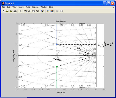
Geometrically these variables are represented in the fig.

4.11.

Trigonometrically it can be derived that the magnitude of the complex poles

corresponds to and the phase, α, is , i.e.

. Thus, given a

second-order system expressed as in (4.30) one can guess the position of its poles

()

sasa

()

ωω

nn d

ss j j

ωω

σω

=− ± − =− ±

cos ( )

−

cos( )

4.2

System Transient Re

Fig. 4.11 Graphical meanin

quickly according to th

previously commented:

1. > 1

When > 1, Expre

of the system are

Remembering that

> 1 is called over

2. = 1

When = 1, the ra

real and equal; we a

damped.

3. 0> < 1

In this case, poles

overdamped.

4. = 0

This is an extreme

reaching the stability

to assure the stabili

system can be seen i

sponse

of the parameters ξ, ω

, and ω

values of and distinguishing the three cas

sion (4.32) turns into two real numbers, that is, the pol

eal and different, and thus we are in the first ca

is known as damping ratio, second-order system wi

amped.

ical of Expression (4.32) is zero, and thus the poles a

e in the second case. These systems are called critica

are complex conjugates, and the system is call

case where poles are located at the imaginary ax

limit (remember that real part of poles has to be negati

y of the system). In this situation, the response of t

fig. 4.12.

102 4 System Response Analysis

Example 4.5

Design a transfer function of a second order system with

= 0 and obtain its time

response against a unitary step input.

Solution

Assuming

= 0 in the the general form of the transfer function of a second order

system given by the equation (4.30), we obtain

For example, for K=1 and , the following Matlab code produces the

system output, depicted in fig. 4.12.

>> s=tf('s');

>> G=10/(s^2+10)

Transfer function:

--------

s^2 + 10

>> step(G)

Fig. 4.12 Second-order system response with = 0.

()

4.2 System Transient Response 103

G=-10*s^2/(10*s^2+5)

Transfer function:

-10 s^2

----------

10 s^2 + 5

>> step(G)

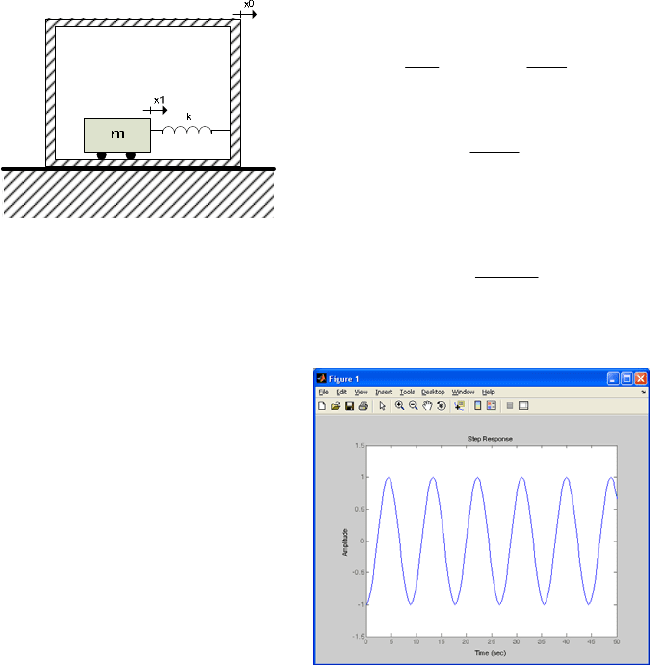
Fig. 4.13 Cart position after a unitary step input. Given that no friction has been modeled,

the cart will never stop.

Example 4.6

Fig. 4.13 a) depicts a cart inside a box and connected to it through a spring. The

box is placed on the ground in such a way that any movement of the ground will

be transmitted to the box and the cart will start to move. It can be considered as a

naïve seismographer. Obtain the transfer function for this system and its step

sponse.

{}

110

10 1 0 1 0

()0

()

() () ()

()

mx k x x

yxx x yx x yx

my mx ky

mkym

dt dt

ms Y s kY s ms X s

ms k

+−=

=−⇒ =+ ⇒ =+

++=

+=−

= ⇒

+=−

−

&& && &&

&& &&

104 4 System Response Analysis

Solution

The equations and the transfer function that model this system are given in

fig. 4.13 b) while fig. 4.13 c-d) depicts the step response of the system and the

Matlab code. The reader will be wondering why the cart is eternally oscillating

when the input has been a unitary step. The answer is simple; in this example cart

friction has not been considered and thus is moving indefinitely since no forces

counteract the movement.

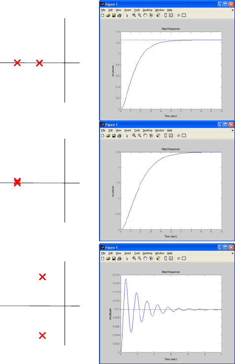
To sum up, the fig. 4.14 entails the exposed casuistry for second-order systems

Overdamped

(

ξ>1)

Critically-damped

(

ξ=1)

Underdamped

(0>

ξ>1)

Fig. 4.14 Typical responses for second-order systems according to the value of ξ.

jω

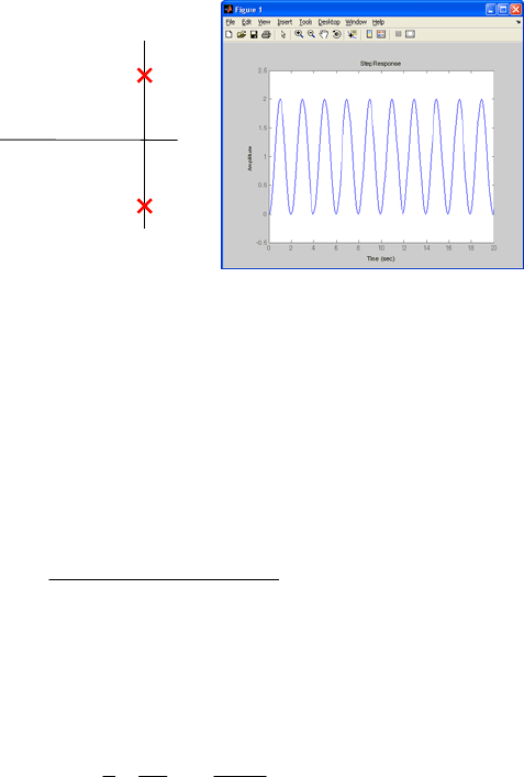
4.2 System Transient Response 105

Underdamped

ξ=0

Fig. 4.14 (continued)

Higher-Order System Response

Unfortunately (or not), real systems are not so trivial than first- or second-order

systems and the study of their responses cannot be described in detail as we did in

the previous section. The casuistry will depend obviously on the order of the

system, i.e. the number of poles, and the number of zeroes. However, a generalized

study can be derived. In general, an n-order-system can be represented as:

(4.33)

Without thoroughness loss, we can assume that the n poles of the transfer function

(4.33) are real and different and that the input signal is a unitary step. With these

assumptions the response Y(s) can be separated as:

(4.34)

which yields the temporal expression

(4.35)

Note that the response of a second-order system with real and different poles is a

particular case of Expression (4.35), that is, assuming p

>0, the system output will

tend to the final value K

. The transient response will depend on the magnitude of

the poles and the values of the coefficients K

jω

( )( )...( )

()

( )( )...( )

Ks z s z s z

spsp sp

++ +

() ()

Ys Gs

ss sp

==+

∑

() ( ) ()

yt K Ke u t

−

∑

106 4 System Response Analysis

When analyzing high-order systems the concept of dominance of poles appears.

It can be said that pole p

dominates pole p

if the following rule yields

(4.36)

Example 4.7

Given a second-order system with poles at p

=1 and p

=10. Determine which pole

is the dominant one.

Solution

The pole p

=1 dominates p

=10 and therefore the effect of the latter on the

response can be insignificant.

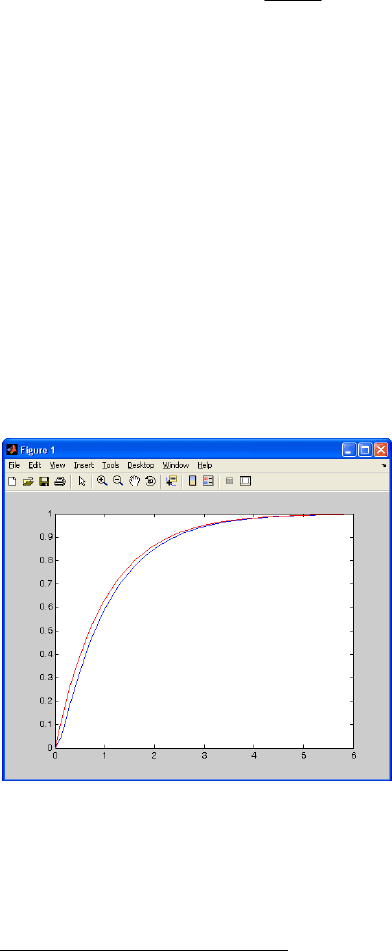
Fig.

4.15 illustrates this example. It depicts the response of a first-order system

with p

=1 (in red) and the response of a second-order system with p

=1 and p

=10.

Notice that the effect of p

is insignificant and the second-order system can be

considered as a first-order one, neglecting p

Through the dominance of poles we can, when applicable, reduce the order of

systems and thus facilitating its study.

>> s=tf('s');

>> G=10/( (s+1)*(s+10))

>> G2=1/(s+1)

>> [x,y]=step(G);

>> [x2,y2]=step(G2);

>> plot(y,x)

>> hold on

>> plot(y2,x2,'r')

Fig. 4.15 Dominance of poles. The response of the second-order system with poles at s=-1

and s=-10 (blue) is quite similar to the one of a first-order system with a pole at s=-1 (red).

This is due to the slight contribution of the pole s=-10 in comparison with the one at s=-1,

which is called a dominant pole in this case.

In absence of zeroes near p

or p

Re( )

4.3 Root Locus 107

In the general case of dealing with conjugate complex poles, similar

considerations are applicable.

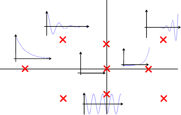
Fig.

4.16 shows the contribution to poles in the response to a high-order system

according to their relative position. The final output will be the sum of their

contribution along the time.

Fig. 4.16 Contribution of poles according to their relative position at the s-plane. Notice

that poles located at the right part of the s-plane produce unstable contributions (tending to

infinite).

4.3 Root Locus

Previous sections have highlighted the particular contribution of poles of a system

according to their position. Thus, when analyzing the response of a given system

we can infer its order and the position of its poles. In a certain way, we are now

interested on the opposite: we want to change the response of a given system, i.e.

its behavior, by moving its poles as desired. To do that we rely on a close-loop

configuration including a parameter whose value will alter the original system.

The root locus technique was proposed by Evans in 1948 as a graphical

representation of the position of the poles of a close-loop system according to the

variations of a system parameter. The general configuration is shown in fig. 4.17,

where the output of the system G(s) is compared to the input, through the H(s)

system. The error E(s), i.e. the difference between the input and the meassured

output, is modulated by the parameter K, being E(s)*K the input of G(s).

jω