Canete J.F. System Engineering and Automation: An Interactive Educational Approach
Подождите немного. Документ загружается.

168 6 System Simulation
Continuous-time systems must undergo a process of discretization that
transforms the governing differential equations in discrete equations. They use
numerical integration methods, whose aim is the replacement of the derivatives of
system variables by approximate expressions.
In general, we are going to consider nth-order system represented by a set of n
state variable equations, as follows
,
,
(6.1)
where and represent the state vector and the input vector respectively,
and
,
is, in general, a non-linear function, and represents the dynamic
model that approximates the behavior of the system under study.
The objective of the simulation techniques is obtaining a sequence of values of
the state vector
,
,…,
,
which approximates the solution of
the ordinary differential equation (ODE) system in fig. 6.1, by using the parameter
defined as integration step is given by
.
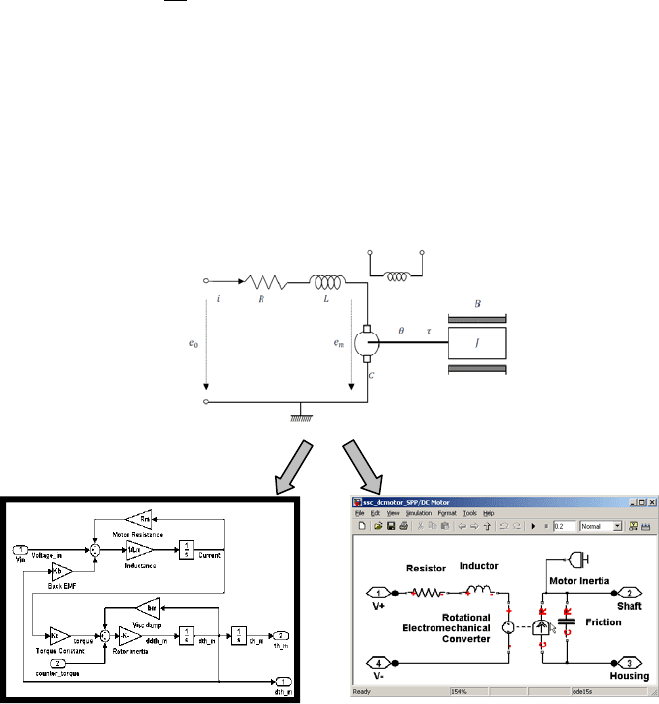
(a) (b)
Fig. 6.1 Computer simulation of a DC motor by using (a) SIMULINK and (b) SIMSCAPE
6.2 Numerical Methods 169
A computer simulation must embody several components. In first place, the
structure of the dynamic model to be simulated must be known, as also the set of
model parameters and initial conditions. In second place, the set of input signals
must also be embodied, and a set of output signals must be explicitly defined in
order to follow the system evolution. Finally, a simulation run time control system
must be included in order to select the numerical integration method used and the
value of its associated parameters, integration step, error tolerances, etc. We will
particularize the computer simulation task by employing simulation software as
SIMULINK or SIMSCAPE, using both block diagrams and physical elements
interconnected to synthesize the model equations (fig. 6.1).
6.2 Numerical Methods
The solution of ordinary differential equations (ODEs) on a digital computer
involves numerical integration. These techniques can be grouped into two broad
classes, termed explicit and implicit integration methods.
Common to all these methods, the resolution of the ordinary differential
equations which describe the system dynamics of (6.1) by integration between
points
and
as
,
(6.2)
,
(6.3)
where
indicates the actual simulation time, while the index denotes the
number of integration steps used to approximate this integral.
Based on the approximation of
,
in the interval of integration and the
number of integration steps selected, arise the different integration methods.
6.2.1 Explicit Numerical Methods
These numerical methods characterized by the state variable
in (6.3) is a
function of the variable values at step and earlier. These methods are
straightforward and easy to program, but present as a major disadvantage that a
small step size must be used so that the solution converge.
Among these methods, the best known is the method of explicit Euler, given by
the recursive equation
,
,
(6.4)
170 6 System Simulation
which assumes that the function is constant
,
,
for
, and only one integration step (0 is used to approximate this integral.
Also belong to this family the Runge–Kutta methods, characterized by
evaluating the
values at intermediate points inside de integration step. The
number of points used in each step of integration determines the order of method.
The most common version of the method uses four points in each integration step
to approximate the integral in (6.3), and is given by
1
6
1
3
1
3
1
6
(6.5)
,
2
,
2
2
,
2
,
(6.6)
6.2.2 Implicit Numerical Methods
These numerical methods are characterized by the state variable
in (6.3) is
a function of the variable values at step 1 and earlier. These methods lead to
the resolution of non-linear implicit equations for obtaining the
values,
which implies an additional computational effort, although they account for
greater stability in the convergence of the solution.
In the same way as we described formerly, the best known is the method of
implicit Euler, given by the recursive equation
,
(6.7)
which assumes that the function is constant
,
,
for
, and only one integration step (0 is used to approximate this
integral.
6.2 Numerical Methods 171
Table 6.1 List of both explicit and implicit Runge-Kutta numerical methods
Integration Method Algorithm
Runge–Kutta 1 (Explicit Euler)
,
Rung–Kutta 2 Explicit (Heun)
,
2
,
2
2
2
Rung–Kutta 4 Explicit
,
2
,
2
2
,
2
,
1
6
1
3
1
3
1
6
Rung–Kutta 1 (Implicit Euler)
,
Rung–Kutta 2 Implicit (Trapezoidal)
,
2
,
2
2
In the same way, there exist implicit Runge-Kutta methods characterized by
evaluating the
values at intermediate points inside the integration step,
including the
,
value.

172 6 System Simulation
In table 1 are listed with both the explicit and the implicit Runge-Kutta methods
commonly used for different orders (RK-n) depending on the number of points to
be used to approximate the integral.
Example 6.1
Derive the approximate solution corresponding to the dynamical equation given
by
by applying both the explicit and implicit Euler method. Simulate the system by
using both methods in SIMULINK for varying integration steps of 0.5, 1
and 2 for 1, also comparing them with the exact solution
.
Solution
Applying (6.4) for
we get
1
Writing this equation in terms of the initial condition
, and solving iteratively
we obtain the solution points for the explicit solution
1
which will be stable only if 1.
Following the same approach, applying (6.7)
we have
1
1
Writing this equation in terms of the initial condition
, and solving iteratively
we obtain the solution points for the implicit solution
1
1
which will be stable no matter the value for be selected.
6.2 Numerical Methods 173
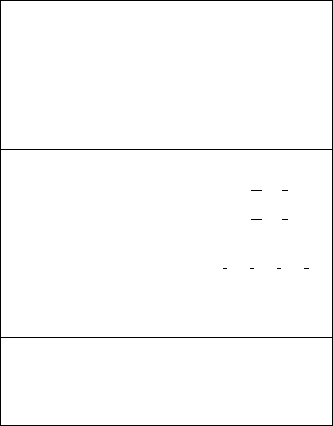
In fig. 6.2 it is shown the simulation diagram corresponding to the dynamis
system defined in this example. The output responses for x
0
4 are shown in
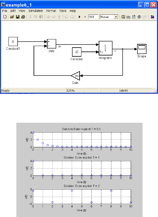
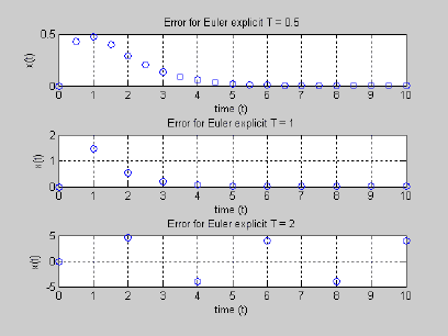
fig. 6.3 for increasing values of T0.5, T1 and T2 for the system
numerically integrated using explicit Euler (‘ode1’ in SIMULINK). It can be
shown how the approximated solution diverges from the exact solution as long as
µTT1 (fig. 6.4).
Fig. 6.2 SIMULINK diagram corresponding to example 6.1.
Fig. 6.3 Output response obtained by using the explicit Euler method for varying T.
174 6 System Simulation
Fig. 6.4 Output error obtained by using the explicit Euler method for varying T.
6.2.3 Multistep Numerical Methods
Multistep methods are characterized by the state variable
in (6.3) is a
function of the variable values
,
,…,
. These methods can be
grouped in a similar way as we did before, in explicit and implicit integration
methods, accounting for the Adams-Bashforth (AB) and Adams-Moulton (AM)
methods. Normally these methods need the solution at several preceding time
points to compute the current solution (‘starting problem’).
In table 6.2 are listed both the explicit AB-n and the implicit AM-n methods
commonly used for different order n, depending on the number of steps to be used
to approximate the integral (for example, ‘ode113’ in SIMULINK with up to 13
steps).
6.2.4 Integration Step Selection
The integration step size must be properly chosen in order to avoid unstabiliy in
the ODE’s solution. In nearly all the cases, there is usually some information
regarding the system time constants. Then, the integration step must be chosen as
¼ of the smallest time constant of the system, in case the integration step is fixed.
However, the integration step can be made variable, depending on the estimated
integration error as the difference in the evaluation of xi +1 with two different
methods in each step of integration, for example RK-4 and RK-5 (‘ode45’ in
SIMULINK) Thus, if the error is less than a tolerance, the step of integration is
increased, and vice versa.

6.2 Numerical Methods 175
Table 6.2 List of both Adams-Bashforth and Adams-Moulton numerical methods
Integration Method Algorithm
Adams-Bashforth 1 (Explicit Euler)
,
Adams-Bashforth 2
,
,
3
2
2
Adams-Bashforth 3
,
,
,
23
12
4
3
5
12
Adams-Moulton 1 (Implicit Euler)
,
Adams-Moulton 2
,
,
2
2
Adams-Moulton 3
,
,
,
5
12
2
3
1
12
In spite of this, some systems exhibit time constants very different from one
another, so that the integration methods or even the variable step size algorithm
described will not work. These systems are called stiff systems.

176 6 System Simulation
A large number of implicit methods are well suited for stiff systems, in
particular the Gear method (’ode15s’ in SIMULINK) and Rosenbrock (’ode23s’ in
SIMULINK).
Table 6.3 Characteristics of the numerical methods handled in SIMULINK
Integration Method Characteristics
Explicit RK-n
(ode1- ode5)
Explicit Runge-Kutta one-step solver, with
fixed integration step. Useful when time constant
is known. More accuracy for higher n values
Explicit RK4-RK5
(ode45)
Explicit Runge-Kutta one-step solver, with
variable integration step. Is the default solver,
and the first method to try for most systems.
Explicit RK2-RK3
(ode23)
Explicit Runge-Kutta one-step solver, with
variable integration step. Is more efficient than
ode45 for coarse tolerances
AB-AM
(ode113)
Adams-Bahforth Adams-Moulton multistep
solver, with variable integration step. Is more
efficient than ode45 for stringent tolerances,
useful when high accuracy is demanded
Gear Method
(ode15s)
Gear based variable order and multistep
solver. Is efficient when some kind of stiffness is
present
Rosenbrock Formula
(ode23s)
Rosenborck order 2 formula one-step solver.
Is efficient when some kind of stiffness is
present and is more efficient than ode23s for
coarse tolerances
The SIMULINK environment incorporates most of the integration methods
presented, both explicit (Runge–Kutta and Adams–Bashfort) and implicit (Gear
and Rosenbrock) including one-step and multistep ones, and table 6.3 shows the
main characteristics of the referred methods.
6.3 Systems Simulation in SIMULINK 177
6.3 Systems Simulation in SIMULINK
SIMULINK is a graphical, block oriented simulation language for modeling and
simulation of dynamics systems. This computer package is an extension to
MATLAB and can also interface with in order to provide it with flexibility.
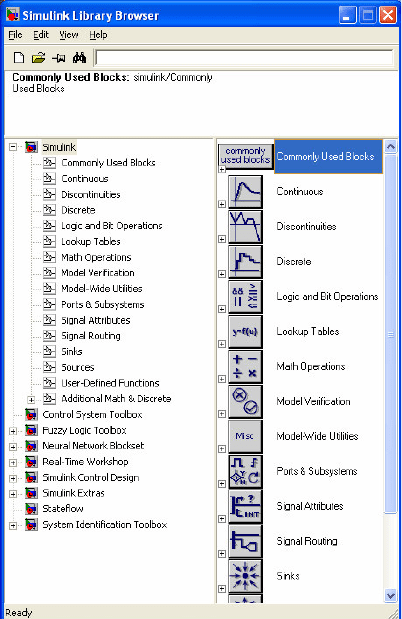
In SIMULINK, systems are drawn on screen as block diagrams by selecting the
basic components from a large library of component blocks, among which we
include continuous, discontinuous, math operators, signal routing, inputs, and
outputs blocks.
Fig. 6.5 The Library browser of the SIMULINK program.
In SIMULINK, a model is a collection of blocks which, in general, represents a
dynamic system. Blocks are used to generate, modify, combine, output, and
display signals, and can be modified by double-clicking on them. Lines are used to
transfer signals from one block to another. These blocks are arranged in Block