Canete J.F. System Engineering and Automation: An Interactive Educational Approach
Подождите немного. Документ загружается.

198 Appendix A: The MATLAB System Control Toolbox
>> A = [0 1;-5 -2];
>> B = [0; 3];
>> C = [1 0];
>> D = 0;
>> H = ss(A,B,C,D)
a =
x1 x2
x1 0 1
x2 -5 -2
b =
u1
x1 0
x2 3
c =
x1 x2
y1 1 0
d =
u1
y1 0
Continuous-time model.
A.5 Access to Model Data
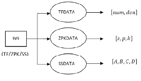
The recovering of data from a system object is made by applying the tfdata,
zpkdata and ssdata commands (fig. A.2), using the format
>> [num,den] = tfdata (sistema, 'v')
>> [z,p,k] = zpkdata(sistema,'v')
>> [A,B,C,D] = ssdata(sistema)
where the argument 'v' enables the return of data vectors instead of arrays of cells.
Fig. A.2 Creation of models for linear time invariant (LTI) systems.
A.6 Building Complex Models 199
Example
Given the SISO transfer function in MATLAB by
>> h = tf([1 1],[1 2 5])
extract the coefficients of the numerator and denominator.
We would have to apply
>> [num,den] = tfdata(h,'v')
num =
0 1 1
den =
1 2 5
A.6 Building Complex Models
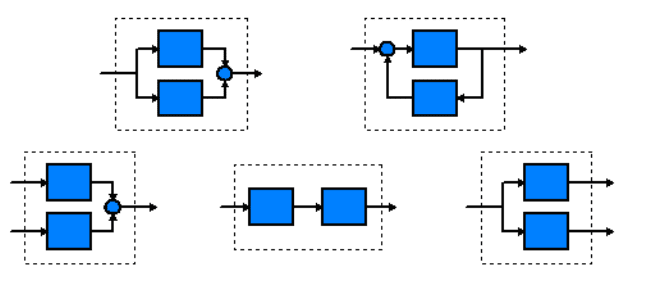
There are a number of functions to help build complex models (fig. A.3), among
which are included:
• Serial and parallel connections (series, parallel)
• Feedback connections (feedback)
• Concatenation ([,], [;] and append)
Fig. A.3 Different connection configurations between models
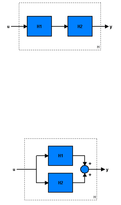
In (fig. A.4) it is shown that the serial connection between the models H1 and
H2, which is realized by using
>> H = series(H1, H2);
or else
>> H = H2 * H1;
200 Appendix A: The MATLAB System Control Toolbox
Fig. A.4 Serial connection configuration
In fig. A.5 it is shown that the parallel connection between the models H1 and
H2, which is realized by using
>> H = parallel(H1, H2);
or else
>> H = H2 + H1;
Fig. A.5 Parallel connection configuration
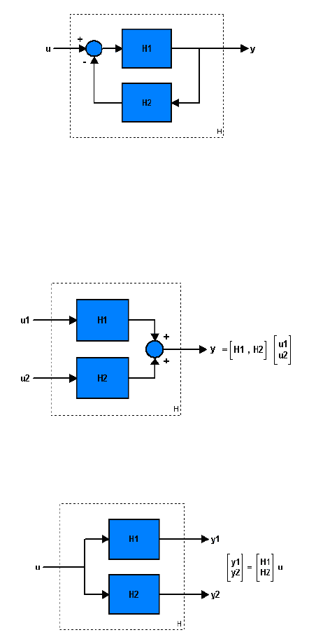
In fig. A.6 it is shown that closed loop configuration between the models H1
and H2 with negative feedback, which is realized by using
>> H = feedback (H1, H2);
The negative feedback is the default option, and if positive feedback is desired, a
‘+’ sign must be specified as
>> H = feedback (H1, H2,+1);
A.6 Building Complex Models 201
Fig. A.6 Closes loop connection configuration
The concatenation of models can be made in different ways (fig. A.7),
(fig. A.8), (fig. A.9):
>> H = [H1,H2];
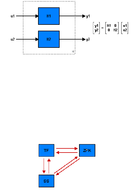
Fig. A.7 Concatenation of models (1 output, 2 inputs)
>> H = [H1; H2];
Fig. A.8 Concatenation of models (2 outputs, 1 input)
>> H = append(H1,H2);
202 Appendix A: The MATLAB System Control Toolbox
Fig. A.9 Concatenation of models (2 outputs, 2 inputs)
A.7 Conversion between Models
LTI models can be converted from one type to another (fig. A.10) by using the tf,
zpk and ss commands,
>> System = tf (system); % TF model converts
>> System = ZPK (system); % ZPK model converts
>> System = ss (system); % converts the SS model
Fig. A.10 Conversion between model formats
Example
>> Gs= ss (-2,1,1,3);
can be converted to zeros, poles, and gain using
>> Gz = zpk(Gs)
Zero/pole/gain:
3 (s+2.333)
-----------
(s+2)
A.8 Time Response
In order to compare the performance of different control systems, different types of
standard test signals are used. This performance is analyzed by using response
characteristics such as settling time, rise time, etc. Besides, the design specifications

A.8 Time Response 203
are often given as a function of the system's response to test signals such as step,
ramp, or parabolic unit impulse. MATLAB incorporates these test signals, generating
also the system response graphs.
The step response of a system can be obtained by application of the step
command
>> step(sys,t)
where
:∆:
is the time horizon, with
, ∆ and
being the initial, step
and final time. Also it is possible to save the step response by using
>> [y,t,x] = step(sys)
The impulse response can be elicited by application of the impulse command
>> impulse(sys,t)
>> [y,t,x] = impulse(sys)
In case of a general input signal
,
:∆:
the system response is
obtained by using the lsim command, so that
>> lsim(sys,u,t)
>>[y,t,x] = lsim(sys,u,t)
Example
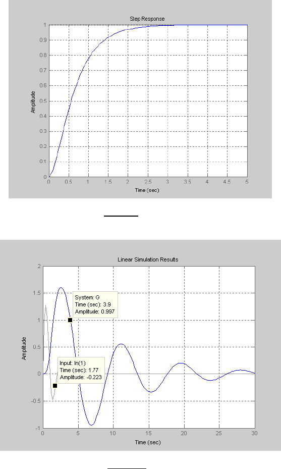
Draw the step response of the system whose function transfer is given by
for 05.
We apply the following list of commands:
>> s=zpk('s');
>> G=10/((s+2)*(s+5));
>> t=0:0.1:5;
>> step(G,t)
>> grid
The step response is plotted in fig. A.11.
Example
Draw the response of the system whose function transfer is given by
for an input signal
2
sin
, 010.
We apply the following list of commands,
>> s=tf('s');
>> G=5/(s^3+2*s^2+s+1);
>> t=0:0.2:30;
204 Appendix A: The MATLAB System Control Toolbox
>> u=2*exp(-t).*sin(pi*t);
>> lsim(G,u,t)
>> grid
The time response for
is plotted in fig. A.12.
Fig. A.11 Step response of
Fig. A.12 Time response for
.

A.8 Time Response 205
Besides this, MATLAB can help to accomplish the partial fraction expansion of
a rational function through the residues calculation.
The command residue finds the residues, poles and direct term of a partial
fraction expansion of the ratio of two polynomials
according to
by applying
>> [K,P,T] = residue(N,D);
Example
Find the poles and residues of
.
>> s=tf('s');
>> C=(2*s+1)/(s^4+3*s^3-7*s+3);
>> [N,D]=tfdata(C,'v');
>> [K,P,T] = residue(N,D)
K =
-0.0270 + 0.1888i
-0.0270 - 0.1888i
0.5000
-0.4460
P =
-2.2428 + 1.0715i
-2.2428 - 1.0715i
1.0000
0.4856
T =
[]

Appendix B:
The rltool Interactive Tutorial
Appe ndix B T he rlto ol Interactive Tutorial
Appendix B
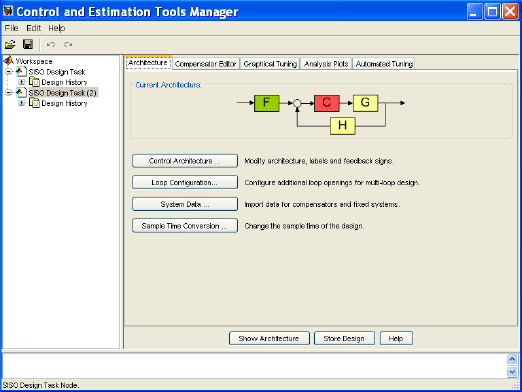
The rltool (‘Root Locus Tool’) is a MATLAB guided user interface (GUI) used to
perform the root locus analysis of linear and invariant single-input single-output
systems.
This application provides a useful tool to realize both the design and the testing
of controllers by using the root locus drawn. In this way, it is possible to change
the gain or to add poles/zeros and see directly the results by viewing the system
response when closed loop poles are moved throughout its root locus.
Fig. B.1 The Control and Estimation Tool Manager of rltool.
The rltool can be executed by typing
>> rltool