Canete J.F. System Engineering and Automation: An Interactive Educational Approach
Подождите немного. Документ загружается.

188 6 System Simulation
Fig. 6.19 Heights
and
for a pulse change for example 6.4
Fig. 6.20 Flowrates
and
for a pulse change for example 6.4.
Example 6.5
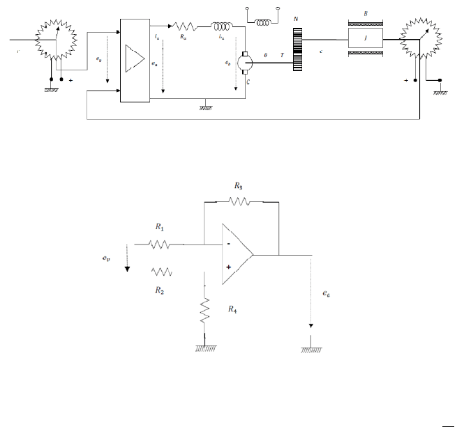
The diagram of fig. 6.21 shows a position servomechanism used for the car
guidance. The aim is to position the mechanical load on ct (wheel angle)
according to the reference position rt (steering wheel angle). For this, two
potentiometers measure the error position, and convert it to an electrical signal
proportional
through the constant
.
A controller based on O.A. amplifies this signal and feeds a DC motor with
resistance
and inductance
. The motor produces a torque
proportional
to the current
through the gain
, and a rotation speed of proportional
through
to the counter-electromotive voltage
. The torque has to
overcome the inertia of the mechanical load and of the engine itself plus the
friction through the gear with ratio .
6.5 Applications 189
The electrical diagram of the O.A. is enclosed in (fig. 6.22), being constituted
by the four resistances
,
,
,
, with an inversion stage included
Fig. 6.21 Diagram of the servomechanism of example 6.5.
Fig. 6.22 Diagram of the controller of example 6.5.
Simulate the servomechanism in SIMSCAPE for parameter values of
,
0.06 ,
0.2,
0.01, 0.0004, 0.005, 100,
1,
10, by using “subsystems” blocks, specifically, controller, motor,
and sensor subsystems, obtaining the output response
for a steering step
command .
Solution
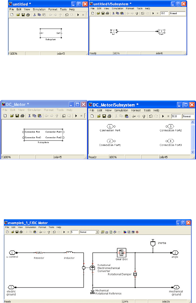
In first place we have to fill up each subsystem block with the constitutive blocks,
starting from an empty block, with a proper number of input and output ports.
These ports have to be added afterwards, by dragging them from the “Utilities
Library” of SIMSCAPE and eliminating at the same time the SIMULINK port
(fig. 6.23).
190 6 System Simulation
Fig. 6.23 Detail of a subsystem block in SIMULINK
In order to model the Motor Subsystem, we need two input ports and two
output ports according to the servomechanism configuration (fig. 6.24).
Fig. 6.24 Transformation of a Subsystem block in SIMSCAPE
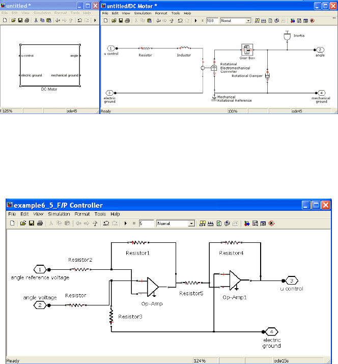
Then, we have to add the necessary blocks which form part of the DC motor,
according to the servomechanism layout. For this task, we will use the Electric
and Mechanical Libraries of SIMSCAPE where these blocks are available
(fig. 6.25 and fig. 6.26).
Fig. 6.25 Elements constitutive of the Motor Subsystem in SIMSCAPE
6.5 Applications 191
Fig. 6.26 Modeling the Motor Subsystem in SIMSCAPE.
In a similar way, we proceed to the modeling of the controller subsystem by
selecting the adequate electric components from the Electric Library (fig. 6.27).
Fig. 6.27 Modeling the Controller Subsystem in SIMSCAPE.
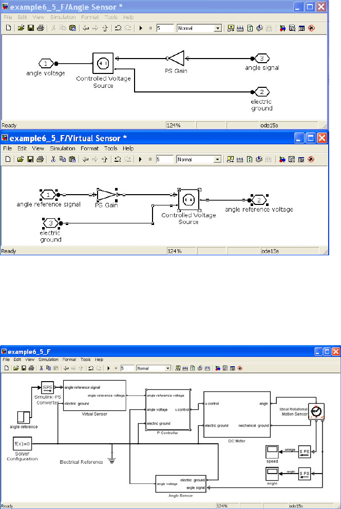
In addition to this, it is also necessary to realize the modeling, both of the angle
sensor and of the inverse angle sensor, in order to convert the wheel angle to
voltage (angle sensor), and the steering wheel angle to reference voltage (virtual
angle sensor) (fig. 6.28).
192 6 System Simulation
Fig. 6.28 Modeling the Angle Sensor and Virtual Angle Sensor Subsystems in SIMSCAPE.
In fig. 6.29 the complete block diagram obtained linking the subsystems
previously modeled following the servomechanism design is shown.
Fig. 6.29 Modeling the complete servomechanism system in SIMSCAPE.
6.5 Applications 193
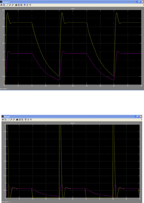
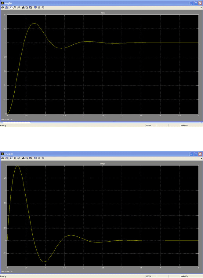
The time response for a unit step reference change in the steering wheel is
depicted in fig. 6.30, showing the adequate tracking for the wheel angle. The step
response is also included in fig. 6.31.
Fig. 6.30 Wheel angle
for a pulse change for example 6.5.
Fig. 6.31 Wheel speed for a pulse change for example 6.5.

Appendix A:
The MATLAB System Control Toolbox
Appendix A The MATLAB Syste m Control Toolb ox
A.1 Creation of Models
The System Control Toolbox of system MATLAB includes commands for
the creation of four basic types of models for linear time invariant (LTI) systems
(fig. A.1):
• Models Transfer Function (TF)
• Models of zeros, poles, and gain (ZPK)
• State space models (SS)
Fig. A.1 Creation of models for linear time invariant (LTI) systems.
These functions take model data as input and return objects that include this
data in single MATLAB variables.
A.2 Transfer Function
A model described as a transfer function (TF) is defined by their polynomial of the
numerator and denominator, that is,
TF ZPK SS
Transfer Function Zeros-Poles-Gain State Space

196 Appendix A: The MATLAB System Control Toolbox
where
,
are the coefficients of the numerator, while
,
,
are the coefficients of the denominator. Both polynomials are specified by a vector
of coefficients
,
and
,
,
.
Therefore, the model can be represented by the transfer function of a SISO
system (Single Input Single Output) by specifying the polynomials for the
numerator and denominator as inputs to the command tf.
Example
210
>> num = [1 0]; % Numerador ->
>> den = [1 2 10]; %Denominador:->
210
>> H = tf (num,den)
Transfer function:
s
--------------
s^2 + 2 s + 10
Alternatively this model can be specified as an expression involving the 's' term by
defining
>> s = tf('s'); % Create Laplace variable
>> H = s/(s^2+2*s+10)
Transfer function:
s
--------------
s^2 + 2 s + 10
In both cases, an object H representing the system model is created in MATLAB.
>> H
Transfer function:
s
--------------
s^2 + 2 s + 10
A.3 Zeros, Poles, and Gain
A model can also be described in the form of zeros, poles and gain (ZPK), which
is a factored form to express a transfer function model, that is
where K is the gain,
are the zeros of and
are the poles of
.
In this format, a model is characterized by its gain value (K), its zeros (which
are the roots of the numerator polynomial) and its poles (which are the roots of the
denominator polynomial) and is represented by using the command zpk.

A.4 State Space 197
Example
2
1
2
22
>> z = [-1]; % Zeros
>> p = [2 1+i 1-i]; % Polos
>> k = 2; % Gain
>> H = zpk(z,p,k)
Zero/pole/gain:
2 (s+1)
---------------------
(s-2) (s^2 - 2s + 2)
Alternatively this model can be specified as an expression involving the 's' term by
defining
>> s = zpk('s');
>> H = 2*(s+1)/((s-2)*(s^2-2*s+2))
Zero/pole/gain:
2 (s+1)
---------------------
(s-2) (s^2 - 2s + 2)
In both cases, an object H representing the system model is created in MATLAB.
>> H
Zero/pole/gain:
2 (s+1)
---------------------
(s-2) (s^2 - 2s + 2)
A.4 State Space
A model can also be described in the form of state space (SS) starting from the
linear differential equations that describe the dynamics of the system. We use the
matrices A, B, C, and D of the state space to characterize this model, in the form
where is the state vector, and are the input and output vectors.
In this format, a model is characterized by the four matrices ,, and ,
being represented by using the command ss, which derives a system object to
represent it.
Example
;
01
5 2
0
3
;
10
0