Canete J.F. System Engineering and Automation: An Interactive Educational Approach

Подождите немного. Документ загружается.

208 Appendix B: The rltool Interactive Tutorial

from the MATLAB command window or else

>> rltool(G)

in case we have created a transfer function ‘G’ previously. In both cases, the

‘Control and Estimation Tool Manager’ is activated, showing the closed loop

configuration actually used, where ‘F’, ‘C’, ‘G’ and ‘H’ stand for filter, controller,

plant and sensor, all of these represented by linear and invariant transfer functions

(fig. B.1)

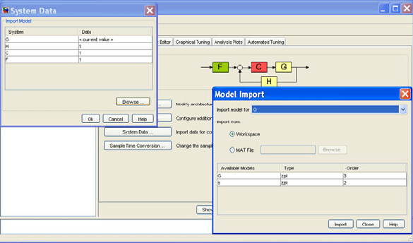
These transfer functions can be imported from the MATLAB command

window if they are previously created by selecting the ‘System Data’ option

(fig. B.2).

Fig. B.2 The selection of closed loop components form the Control and Estimation Tool

Manager’

For instance, if we execute

>> s=zpk('s');

>> G= 5*(s+2)/(s*(s+1)*(s+5));

>> rltool(G)

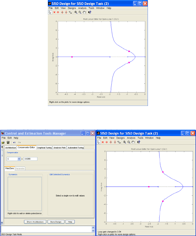
then, the rltool GUI is opened showing the root locus for ‘G’ for the case of

controller compensator C = 1 (fig. B.3). In this chart we can observe the closed

loop pole location as pink squares, which can be moved by dragging them along

the root locus. Note that the controller gain automatically changes in the ’Current

Compensator” window (fig. B.4).

Appendix B: The rltool Interactive Tutorial

209

Fig. B.3 The window design of rltool, showing the root locus plot.

Fig. B.4 The Compensator Editor window of rltool.

This ‘Compensation Editor’ toolbar allows to add poles, add zeros or to delete

either for the controller by selecting the ‘Pole/Zero’ option. This operation can

also be made by right clicking and accessing to the ‘Add Pole/Zero’ or ‘Delete

Pole/Zero’ option.

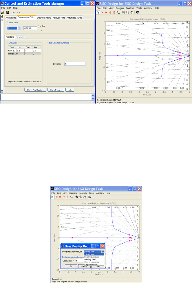
For instance, we can add a zero at s = -0.5 and an integrator at s = 0 we get

another root locus plot with moving closed loop poles (fig. B.5).

210 Appendix B: The rltool Interactive Tutorial

Fig. B.5 The Compensator Editor window of rltool showing the effect of added poles/zeros

It can be seen how this proportional integral controller has moved the root locus

graph to the right half plane, by impairing its transient performance (even causing

unstability) but at the same time improving its steady state regime.

The rltool also enables to super-impose design constraints on the s-plane. For

this, we have to right click and select ”Design Requirements”, then ”New” in the

”Constraint type” menu. It is possible to choice between ‘Settling Time’, ‘Percent

Overshoot’, ‘Damping Ratio’, ‘Natural Frequency’ and ‘Region Constraint’

requirements that can be viewed over an s-grid by right clicking ‘Grid’ (fig. B.6).

Fig. B.6 The Design Requirements setting of rltool

Appendix B: The rltool Interactive Tutorial

211

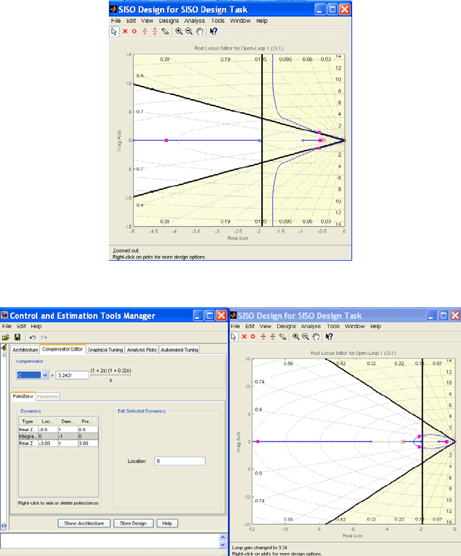
For example, we can select a settling time 



2  and a percent overshoot





20 %. It can be seen that these specifications cannot be met with this

controller, no matter what we set the proportional gain to. That is, the

two dominant roots of the closed loop system will never be in the valid region

(fig. B.7).

Fig. B.7 Imposing specific requirements in rltool

Fig. B.8 Fulfilling requirements by modifying the controller in rltool

Nevertheless, we can add a new the controller zero by using the toolbar in the

rltool main window and drag one of the closed loop poles until they are inside the

212 Appendix B: The rltool Interactive Tutorial

white region. Note how the new compensator transfer function designed meets the

requirements in spite of the closed loop pole closer to the zero at s= -0.5 due to the

cancellation effects (fig. B.8).

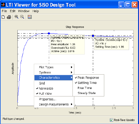
Besides we can see the time responses of the closed loop system by selecting

the ‘Analysis’ at the toolbar and the ‘Response to Step Command option. Then, a

new plot window is opened, showing the step response from the reference to the

system’s output (fig. B.9). By right clicking, it can be shown that the time

response characteristics (peak response, settling time, etc.) in order to test if the

requirements have been effectively met.

Fig. B.9 Step response of the closed loop system designed by rltool

Appendix C:

The SIMULINK Interactive Tutorial

Appendix C The SIMULINK Interactive Tutorial

Appendix C

C.1 Introduction

SIMULINK is an extension to MATLAB that allows users to rapidly and

accurately build computer models of dynamical systems using block diagrams.

A block diagram describes a set of relationships that holds simultaneously, so the

block diagram can be thought of being represented by a set of simultaneous equations.

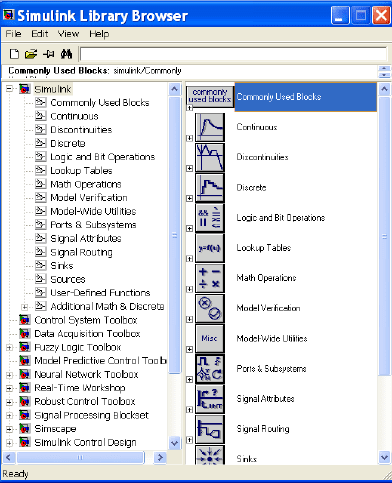
The block diagram is assembled by gathering the constitutive blocks from the

SIMULINK Library Browser, which are grouped by categories into different

libraries (fig. C.1).

Fig. C.1 The SIMULINK Library browser

214 Appendix C: The SIMULINK Interactive Tutorial

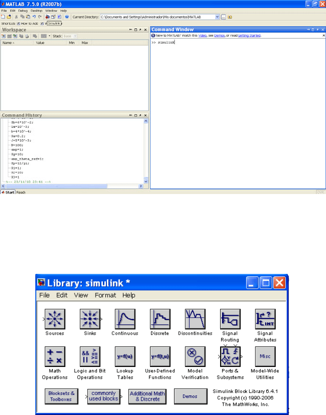
In order to access SIMULINK we can type in the MATLAB command window

>> SIMULINK

or else click on the SIMULINK icon (fig. C.2)

Fig. C.2 The access to SIMULINK from MATLAB

Once we access SIMULINK a new model must be created by dragging blocks

from the SIMULINK Library browser to this new model window, by selecting the

appropriate library where the searched block is included.

Fig. C.3 The SIMULINK Block Library

For the purpose of modeling, simulation, and control of dynamic systems, a subset

of SIMULINK libraries will be used, namely, Continuous, Discontinuities, Lookup

C.2 Creating a Model 215

Tables, Math Operations, Ports and Subsystems, Signal Routing, Sinks, Sources, User-

Defined Functions and Additional Linear (included into SIMULINK Extras) (fig. C.3)

C.2 Creating a Model

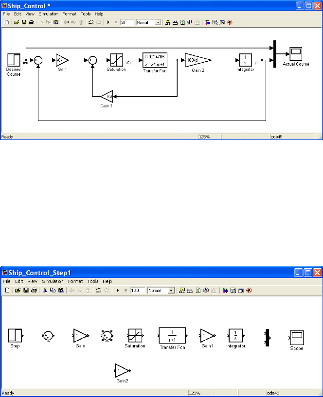
In order to explain the process followed to create a SIMULINK model, we have

selected a simple feedback control system for a ship (fig. C.4).

Fig. C.4 Feedback control system for a ship

In the first place we have to collect all blocks necessary to build the system from the

SIMULINK block Library. Afterwards, we will connect the selected blocks to

implement the block diagram, also changing the parameters of these blocks if it is

necessary. Finally the system is simulated by selecting the appropriate solver options.

Therefore, as first step, we open a new model, dragging the constitutive blocks

of the block diagram from each one of the block libraries where they are included

(fig. C.5)

Fig. C.5 Building process for the feedback control of a ship (step 1)

216 Appendix C: The SIMULINK Interactive Tutorial

As second step, we connect these blocks following the desired connection

pattern as indicated in the feedback control system (fig. C.6). Possibly, it will be

necessary to flip or rotate some blocks or to derive some pickoff points.

Fig. C.6 Building process for the feedback control of a ship (step 2)

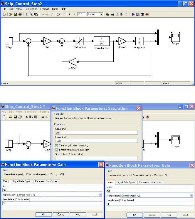
Fig. C.7 Building process for the feedback control of a ship (step 3)

Afterword, in a third step we have to change the block’s parameters according

to the values defined in the original feedback control system if it is necessary,

adding optionally labels both to identify the signals transferred between blocks or

to name specific blocks (fig. C.7). Block parameters can also be defined from the

MATLAB workspace and used in SIMULINK. In this case we have assigned the

gains, maxim saturation, and reference step as

>> Kd=1.8;

>> Kp=1.5;

C.2 Creating a Model 217

>> Lsat=10;

>> phir=90;

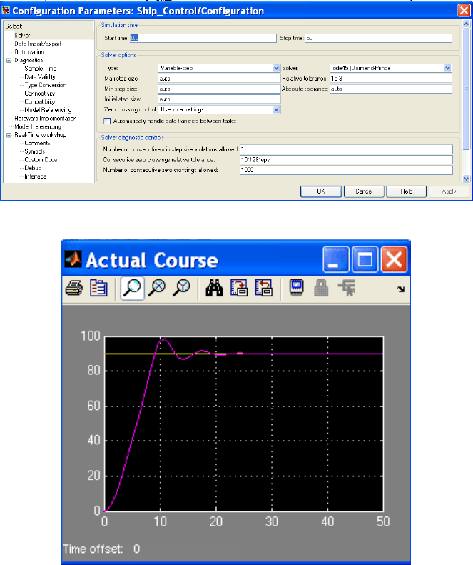
Before simulation is run, we must select the appropriate simulation time and the

numerical method used, including the integration step value in case of fixed-step

selection (fig. C.8).

Fig. C.8 Definition of the solver configuration for the feedback control.

Fig. C.9 Step response of the DC motor obtained by using SIMULINK

Finally, the simulation is run by double-clicking on the  icon and output

responses can be viewed by double-clicking on the Scope block to view its output.

Hit the auto-scale button to see the step response of the feedback controller

applied to a reference course for a step amplitude of 90



(fig. C.9)