Devore J.L., Berk K.N. Modern Mathematical Statistics with Applications

Подождите немного. Документ загружается.

THE F TEST

FOR EQUA-

LITY OF

VARIANCES

Null hypothesis:

: s

¼ s

Test statistic value: f ¼ s

Alternative Hypothesis Rejection Region for a Level a Test

: s

> s

f  F

a,m1,n1

: s

< s

f  F

a,m1,n1

: s

6¼ s

either f  F

a/2,m1,n1

or f  F

1a/2,m1,n1

Since critical values are tabled only for a ¼ .10, .05, .01, and .001, the two -

tailed test can be performed only at levels .20, .10, .02, and .002. More

extensive tabulations of F critical values are available elsewhere, including

calculators and computer software.

Example 10.14 Is there less variation in weights of some baked goods than others? Here are the

weights (in grams) for a sample of Bruegger’s bagels (their Iowa City shop) and

another sample of Wolferman’s muffins (made in Kansas City):

B: 99.8 105.4 94.7 107.8 114.3 106.3

W: 99.0 98.2 98.1 102.1 102.9 104.1 98.8 99.5

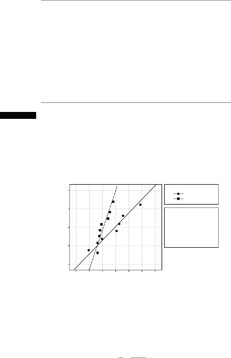
The normality assumption is very important for the use of Expression (10.8)sowe

check the normal plot from MINITAB, shown in Figure 10.9. There is no apparent

reason to doubt normality here.

Notice the difference in slopes for the two sources. This suggests different

variabilities because the vertical axis is the z-score and is related to the horizontal

axis (grams) by z ¼ (grams  mean)/(std dev). Th us, when score is plotted against

grams the slope is the reciprocal of the standard deviation. Now let’s test

¼ s

against a two-tailed alternative with a ¼ .02. We need the critical values

.01,5,7

¼ 7.46 and F

.99,5,7

¼ 1/F

.01,7,5

¼ 1/10.46 ¼ .0956. We have

f ¼

6:765

2:338

¼ 8:37

90 95 100 105 110 115 120

grams

−1

−2

Score

brand

bruegger's

wolferman's

Mean

104.7

100.3

StDev

6.765

2.338

0.206

0.548

0.762

0.107

Figure 10.9 Normal plot for baked goods

528

CHAPTER 10 Inferences Based on Two Samples

which exceeds 7.46, so the hypothesis of equal variances is rejected. We conclude that

there is a difference in weight variation, and the English muffins are less variable.

Notice that it is not really necessary to use the lower-tailed critical value here if

the groups are chosen so the first group has the larger variance, and therefore the

value of f ¼ s



exceeds 1. Because f > 1, the only comparison is between the

computed f and the upper critical value 7.46. It does not change the result of the test to

fix things so f > 1, so it is not cheating to simplify the test in this way.

■

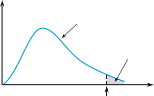
P-Values for F Tests

Recall that the P -value for an upper-tailed t test is the area under the relevant t curve

(the one with appropriate df) to the right of the calculated t. In the sam e way, the

P-value for an upper-tailed F test is the area under the F curve with appropriate

numerator and denominator df to the right of the calculated f. Figure 10.10 illus-

trates this for a test based on n

¼ 4 and n

¼ 6.

Unfortunately, tabulation of F curve upper-tail areas is much more cumber-

some than for t curves because two df’s are involved. For each combination of n

and n

, our F table gives only the four critical values that capture areas .10, .05, .01,

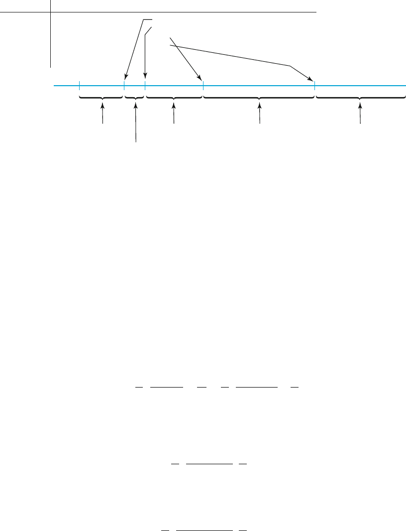
and .001. Figure 10.11 (next page) shows what can be said about the P-value

depending on where f falls relative to the four critical values.

For example, for a test with n

¼ 4 and n

¼ 6,

f ¼ 5.70 ) .01 < P-value < .05

f ¼ 2.16 ) P-value > .10

f ¼ 25.03 ) P-value < .001

Only if f equals a tabulated value do we obtain an exact P-value (e.g., if f ¼ 4.53,

then P-value ¼ .05). Once we know that .01 < P-value < .05,

would be

rejected at a significance level of .05 but not at a level of .01. When P-value

< .001,

should be rejected at any reasonable significance level.

The F tests discussed in succeeding chapters will all be upper-tailed.

If, however, a lower-tailed F test is appropriate, then (6.15) should be used to

obtain lower-tailed critical values so that a bound or bounds on the P-value can

be established. In the case of a two-tailed test, the bound or bounds from a one-

tailed test should be multiplied by 2. For example, if f ¼ 5.82 when n

¼ 4 and

¼ 6, then since 5.82 falls between the .05 and .01 critical values, 2(.01) < P-

value < 2(.05), giving .02 < P-value < .10.

would then be rejected if a ¼ .10

f = 6.23

F curve for

= 4, v

= 6

Shaded area = P-value

= .025

Figure 10.10 A P-value for an upper-tailed F test

10.5 Inferences About Two Population Variances 529

but not if a ¼ .01. In this case, we cannot say from our table what conclusion is

appropriate when a ¼ .05 (since we don’t know whether the P-value is smaller or

larger than this). However, statistical software shows that the area to the right of

5.82 under this F curve is .029, so the P-value is .058 and the null hypothesis should

therefore not be rejected at level .05 (.058 is the smallest a for which

can be

rejected and our chosen a is smaller than this).

A Conﬁdence Interval for s

The CI for s

is based on replacing F in the probability statement

PðF

1a=2;n

< F < F

a=2;n

Þ¼1  a

by the F variable (10.8) and manipulating the inequalities to isolate s



a=2;n



1a=2;n

 F

a=2;n

Equation (6.15 ) has been used here to simplify the upper bound and enable use of

Table A.8. Thus the confidence interval for s



a=2;m1;n1

;

 F

a=2;n1;m1



An interval for s

results from taking the square root of each limit:



ﬃﬃﬃﬃﬃﬃﬃﬃﬃﬃﬃﬃﬃﬃﬃﬃﬃﬃﬃﬃﬃﬃﬃ

a=2;m1;n1

;



ﬃﬃﬃﬃﬃﬃﬃﬃﬃﬃﬃﬃﬃﬃﬃﬃﬃﬃﬃﬃﬃﬃﬃ

a=2;n1;m1

In the interval for the ratio of population variances, notice that the limits of the

interval are proportional to the ratio of sample variances. Of course, the lower limit

is less than the ratio of sample variances, and the upper limit is greater.

1 . . .

4 . . .

6 .10

.05

.01

.001

3.18

4.53

9.15

21.92

P-value

> .10 P-value < .001.01 <P-value < .05 .001 < P-value < .01

.05

< P-value < .10

Figure 10.11 Obtaining P-value information from the F table for an upper-tailed F test

530

CHAPTER 10 Inferences Based on Two Samples

Example 10.15 Let’s find a confidence interval using the data of Example 10.14. The sample

standard deviations are s

¼ 6.765 for 6 Bruegger’s bagels, and s

¼ 2.338 for

8 Wolferman English muffins. Then a 98% confidence interval for the ratio s

6:765

2:338



ﬃﬃﬃﬃﬃﬃﬃﬃﬃﬃﬃﬃﬃ

:01;5;7

;

6:765

2:338



ﬃﬃﬃﬃﬃﬃﬃﬃﬃﬃﬃﬃﬃ

:01;7;5



¼ 2:89 

ﬃﬃﬃﬃﬃﬃﬃﬃﬃ

7:46

; 2:89 

ﬃﬃﬃﬃﬃﬃﬃﬃﬃﬃﬃ

10:46



¼ð1:06; 9:35Þ

Because 1 is not included in the interval, it sugges ts that the two standard deviations

differ. By comparing the CI calculation with the hypothesis test calculation, it

should be clear that a two-tailed test would reject equality at the 2% level, and this

is consistent with the results of Example 10.14.

■

It is important to emphasize that the methods of thi s section are strongly

dependent on the normality assumption. Expression 10.8 is valid only in the case of

normal data or nearly normal data. Otherwise, the F distribution in (10.8) does not

apply. The t procedures of this chapter are robust to the normality assumption,

meaning that the procedure s still work in the case of moderate departures from

normality, but this is not true for comparison of variances based on (10.8).

Exercises Section 10.5 (60–68)

60. Obtain or compute the following quantities:

a. F

.05,5,8

b. F

.05,8,5

c. F

.95,5,8

d. F

.95,8,5

e. The 99th percentile of the F distribution with

¼ 10, n

¼ 12

f. The 1st percentile of the F distribution with

¼ 10, n

¼ 12

g. P(F  6.16) for n

¼ 6, n

¼ 4

h. P(.177  F  4.74) for n

¼ 10, n

¼ 5

61. Give as much information as you can about the

P-value of the F test in each of the following

situations:

a. n

¼ 5, n

¼ 10, upper-tailed test, f ¼ 4.75

b. n

¼ 5, n

¼ 10, upper-tailed test, f ¼ 2.00

c. n

¼ 5, n

¼ 10, two-tailed test, f ¼ 5.64

d. n

¼ 5, n

¼ 10, lower-tailed test, f ¼ .200

e. n

¼ 35, n

¼ 20, upper-tailed test, f ¼ 3.24

62. Return to the data on maximum lean angle given

in Exercise 27 of this chapter. Carry out a test at

significance level .10 to see whether the popula-

tion standard deviations for the two age groups are

different (normal probability plots support the

necessary normality assumption).

63. Refer to Example 10.7. Does the data suggest that

the standard deviation of the strength distribution for

fused specimens is smaller than that for not-fused

specimens? Carry out a test at significance level .01

by obtaining as much information as you can about

the P-value.

64. Toxaphene is an insecticide that has been identi-

fied as a pollutant in the Great Lakes ecosystem.

To investigate the effect of toxaphene exposure

on animals, groups of rats were given toxaphene in

their diet. The article “Reproduction Study of

Toxaphene in the Rat” (J. Envir. Sci. Health,

1988: 101–126) reports weight gains (in grams)

for rats given a low dose (4 ppm) and for control

rats whose diet did not include the insecticide. The

sample standard deviation for 23 female control

rats was 32 g and for 20 female low-dose rats was

54 g. Does this data suggest that there is more

variability in low-dose weight gains than in con-

trol weight gains? Assuming normality, carry out

a test of hypotheses at significance level .05.

65. In a study of copper deficiency in cattle, the copper

values (mg/100 mL blood) were determined both

for cattle grazing in an area known to have well-

defined molybdenum anomalies (metal values in

excess of the normal range of regional variation)

and for cattle grazing in a nonanomalous area (“An

Investigation into Copper Deficiency in Cattle in

the Southern Pennines,” J. Agric. Soc. Cambridge,

1972: 157–163), resulting in s

¼ 21.5 (m ¼ 48)

10.5 Inferences About Two Population Variances 531

for the anomalous condition and s

¼ 19.45

(n ¼ 45) for the nonanomalous condition. Test

for the equality versus inequality of population

variances at significance level .10 by using the

P-value approach.

66. The article “Enhancement of Compressive Proper-

ties of Failed Concrete Cylinders with Polymer Im-

pregnation” (J. Test. Eval., 1977: 333–337) reports

the following data on impregnated compressive

modulus (psi  10

)whentwodifferentpolymers

were used to repair cracks in failed concrete.

Epoxy 1.75 2.12 2.05 1.97

MMA prepolymer 1.77 1.59 1.70 1.69

Obtain a 90% confidence interval for the ratio of

variances.

67. Reconsider the data of Example 10.6, and calculate

a 95% upper confidence bound for the ratio of the

standard deviation of the triacetate porosity distri-

bution to that of the cotton porosity distribution.

68. For the data of Exercise 27 find a 90% confidence

interval for the ratio of population standard devia-

tions, and relate your CI to the test of Exercise 62.

10.6

Comparisons Using the Bootstrap

and Permutation Methods

In this chapter we have discussed how to make comparisons based on normal data.

We have also considered comparisons of means whe n the sample sizes are large

enough for the means to be approximately normal. What about all other cases,

especially small skewed data sets?

We now consider the bootstrap technique for forming confidence intervals

and permutat ion tests for testing hypotheses. As described in Section 8.5, boot-

strapping involves a lot of computation. The same will be true here for bootstrap

confidence intervals and for permutation tests.

The Bootstrap for Two Samples

The bootstrap for two samples is similar to the one-sample bootstrap of Section 8.5,

except that samples with replacement are taken from the two groups separately.

That is, a sample is taken from the first group, a separate sample is taken from the

second group, and then the difference of means or some other comparison statistic

is computed. Th is process is repeated until there are 999 (or another large number)

values of the comparison statistic, and this constitutes the bootstrap sample. The

distribution of the bootstrap sample is called the bootstrap distribution.

If the bootstrap distribution appears normal, then a confidence interval can be

computed by using the standard deviation of the bootstrap distribution in place of

the square root expression in the theorem of Section 10.2. That is, instead of

estimating the standard error for the difference of means from the two sample

standard deviations, we use the standard deviation of the bootstrap distribution. The

idea is that the bootstrap distribution should represent the actual sampling distribu-

tion for the difference of means.

However, if the bootstrap distribution does not look normal, then the percen-

tile interval should be calculated, just as was done in Section 8.5. Assuming a

bootstrap sample of size 999, this involves sorting the 999 boots trap values, finding

the 25th from the bottom and the 25th from the top, and using these values as

confidence limits for a 95% CI. The bias corrected and adjusted interval is a further

refinement available in some software, including R, Stata, and Systat.

532 CHAPTER 10 Inferences Based on Two Samples

Example 10.16 As an example of the bootstrap for two samples, consider data from a study of

children talking to themselves (private speech), introduced in Example 1.2. The

children were each observed in many 10-s intervals (about 100) and the researchers

computed the percentage of intervals in which private speech occurred. Because

private speech tends to occur when there is a challenging task, the students were

observed when they were doing arithmetic. The private speech is classified as on

task if it is about arithmetic, off task if it is about something else, and mumbling if

the subject is not clear.

Each child was observed in the first, second, and third grades, but we will

consider here just the first grade off-task private speech. For the 18 boys and

15 girls here are the percentages:

B: 4.9, 5.5, 6.5, 0.0, 0.0, 3.0, 2.8, 6.4, 1.0, 0.9, 0.0, 28.1, 8.7, 1.6, 5.1, 17.0, 4.7, 28.1

G: 0.0, 1.3, 2.2, 0.0, 1.3, 0.0, 0.0, 0.0, 0.0, 3.9, 0.0, 10.1, 5.2, 3.2, 0.0.

With the large number of zeroes, a majority for the girls, the normality assumption

of Section 10.2 does not apply here. Also, the sample sizes for the two groups are

not very large, so the two-sample z methods of Section 10.1 might not work for this

data set. Nevertheless, it is useful to give the t CI for comparison purposes. The

95% interval is

x  y  t

:025;n

ﬃﬃﬃﬃﬃﬃﬃﬃﬃﬃﬃﬃﬃﬃﬃﬃ

¼ 6:906  1:813  2:080

ﬃﬃﬃﬃﬃﬃﬃﬃﬃﬃﬃﬃﬃﬃﬃﬃﬃﬃﬃﬃﬃﬃﬃﬃﬃﬃﬃﬃﬃﬃﬃﬃ

8:719

2:846

¼ 5:093  2:080ð2:1825Þ¼5:093  4:540 ¼ð:55; 9:63Þ

The degrees of freedom n ¼ 21 come from the messy formula in the theorem of

Section 10.2. The confidence interval does not include 0, which implies that we would

reject the hypothesis m

¼ m

against a two-tailed alternative at the .05 level. This is in

agreement with what we get in testing this hypothesis directly: t ¼ 2.33, P-value .030.

The t method is of questionable validity, because of sample sizes that might not

be enough to compensate for the nonnormality. The bootstrap method involves

drawing a random sample of size 18 with replacement from the 18 boys, drawing a

random sample of size 15 with replacement from the 15 girls, and calculating the

difference of means. Then this process is repeated to give a total of 999 differences of

means. The distribution of these 999 differences of means is the bootstrap distribution.

To help clarify the procedure, here are random samples from the boys and girls:

B: 0.0, 3.0, 2.8, 0.9, 3.0, 0.0, 0.0, 6.5, 6.4, 8.7, 6.4, 1.0, 0.9, 5.5, 17.0, 17.0, 0.0, 3.0

G: 1.3, 0.0, 0.0, 0.0, 0.0, 1.3, 1.3, 0.0, 3.2, 0.0, 1.3, 5.2, 0.0, 0.0, 0.0.

Of course, in sampling with replacement some values will occur more than once

and some will not occur at all. For these two samples, the difference of means is

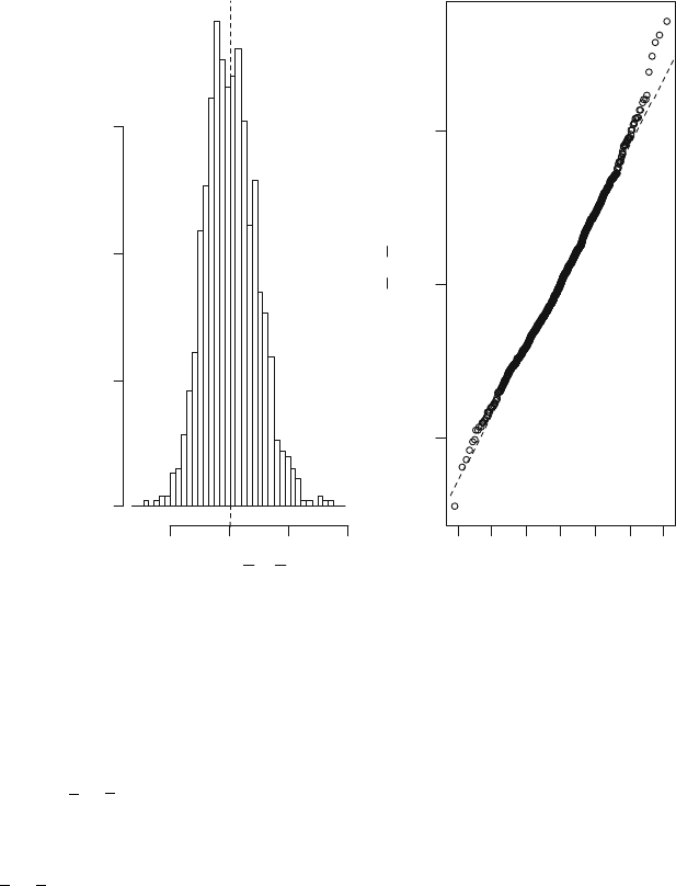
4.56  .91 ¼ 3.65. Doing this 999 times (using the R package boot) gives the

bootstrap distribution displayed in Figure 10.12.

The distribution looks almost normal, but with some positive skewness. The

idea of the bootstrap, with its samples taken from the original samples of boys and

girls, is for this histogram to resemble the true distribution of the difference of means.

If the original samples of boys and girls are representative of their populations, then

our histogram should be a reasonable imitation of the population distribution for the

difference of means.

10.6 Comparisons Using the Bootstrap and Permutation Methods 533

In spite of the nonnormality of the bootstrap distribution, we will use its

standard deviation to compute a confidence interval to see how much it differs from

the perc entile interval. The standard deviation of the bootstrap distribution (i.e., of

the 999

x  y values) is s

boot

¼ 2.1874, very close to the 2.1825 that was computed

for the square root in the t interval above. Using 2.1874 instead of 2.1825 gives the

95% confidence interval

x  y  z

:025

boot

¼ 6:906  1:813  1:96ð2:1874Þ¼5:093  4:287 ¼ð:81; 9:38Þ

This is very similar to the t interval, (.55, 9.63), except that using z

.025

(common bootstrap practice) instead of t

.025,n

shortens the interval. Note that the

R package boot produces a slightly different interval because it replaces the

difference 5.093 with the average of the 999 bootstrap mean differences.

In the presence of a nonnormal bootstrap distribution, we now use the

percentile interval, which for a 95% confidence interval finds the middle 95% of

the bootstrap distribution. The confidence limits for a 95% confidence interval are

the 2.5 percentile and the 97.5 percentile. When the 999 boots trap differences of

means are sorted, the 25th value from the bottom is 1.029 and the 25th value from

the top is 9.760. This gives a 95% CI (1.029, 9.760). The skewness of the bootstrap

distribution pushes the endpoints a little to the right of the endpoints computed from

boot

. In addition, one can compute the bias corrected and accelerated refinement,

as discussed in Section 8.5. The improved interval (1.625, 10.446), obtained from

R, is moved even farther to the right compared to the previous intervals.

■

Density

0 5 10 15

0.00

0.05

0.10

0.15

−3 −2 −10123

Quantiles of Standard Normal

x *–y *

Figure 10.12 Histogram and normal plot of the bootstrapped difference in means

from R

534

CHAPTER 10 Inferences Based on Two Samples

Permutation Tests

How should we test hypotheses when the validi ty of the t test is in doubt?

Permutation tests do not require any specific distribution for the data. The idea

is that under the null hypothesis, every observation has the same distribution and

thus the same expected value, so we can rearrange the group labels without

changing the group population means. We look at all possible arrangements,

compute the difference of means for each of these, and compute a P-value by

seeing how extreme is our original difference of means. That is, the P-value is the

fraction of arrangements that are at least as extreme as the value computed for the

original data.

Example 10.17 Consider a small-scale version of the off-task private speech data. The first three

values for the boys are 4.9, 5.5, 6.5 and the first two values for the girls are 0.0, 1.3.

To demonstrate the permutation test, we will act as if this is the whole data set.

First, we compute the difference of means of the boys versus the girls, 5.63 

.65 ¼ 4.98. Under the null hypothesi s of equal population means, it should not

matter if we reassign boys and girls. Therefore, we consider all ways of selecting

three from among the five observations to be in the boys sample, lea ving the other

two for the girls sample. Unde r the null hypothesis, the following ten choices are

equally likely.

Boys x Girls y x  y

4.9 5.5 6.5 5.63 0.0 1.3 .65 4.98

4.9 5.5 0.0 3.47 6.5 1.3 3.90 .43

4.9 5.5 1.3 3.90 0.0 6.5 3.25 .65

4.9 6.5 0.0 3.80 5.5 1.3 3.40 .40

4.9 6.5 1.3 4.23 5.5 0.0 2.75 1.48

4.9 0.0 1.3 2.07 5.5 6.5 6.00 3.93

5.5 6.5 0.0 4.00 4.9 1.3 3.10 .90

5.5 6.5 1.3 4.43 4.9 0.0 2.45 1.98

5.5 0.0 1.3 2.27 6.5 4.9 5.70 3.43

6.5 0.0 1.3 2.60 5.5 4.9 5.20 2.60

How extreme is our original difference of means (4.98) in this set of ten differ-

ences? Because it is the largest of ten, our P-value for an upper-tailed alternative

hypothesis is

¼ :10. That is, for an upper-tailed test the P-value is the fraction

of arrangements that give a difference at least as large as our original difference.

For a two-tailed test we simply double the one-tailed P-value, giving P ¼ .20 for

this example.

■

When m ¼ 3 and n ¼ 2, it is simple enough to deal with all



¼ 10

arrangements. What happens when we try to use the whole set of 18 boys and 15

girls in the private speech data set?

Example 10.18 Consider a permutation test for the full private speech data. Here we are dealing

with



¼ 1;037;158;320 arrangements of the 18 boys and 15 girls, mor e than a

billion arrangements. Even on a reasonably fast computer it might take a while to

generate this many differences and see how many are at least as big as the value

10.6 Comparisons Using the Bootstrap and Permutation Methods 535

x  y ¼ 6 :906  1:813 ¼ 5:093 computed for the original data. It took around

an hour on an 800 mhz Dell using the free program BLOSSOM, which can be

downloaded from the Internet. The two-tailed P-value is .0203, a little less than the

P-value .030 from the t test. There is fairly strong evidence, at least at the 5% level,

that the boys engage in more off-task private speech than the girls.

We might have expected that the hypothesis test woul d reject the null

hypothesis (of zero difference in means) at the 5% level with a two-tailed test.

Recall that all three of our 95% confidence intervals in Example 10.16 consisted of

only positive values, so none of the intervals included zero.

The number of arrangements goes up very quickly as the group sizes

increase. If there are 20 boys and 20 girls, then the numb er of arrangements is

more than 100 times as big as when there are 18 boys and 15 girls. Doing the test

exactly, using all of the arrangements, becomes entirely impractical, but there is an

approximate alternative. We can take a rando m sample of a few thousand arrange-

ments and get quite close to the exact answer. For example, with our 18 boys and

15 girls, BLOSSOM gives (almost instantaneously) a P-value of .0204, which is

certainly close enough to the exact answer of .0203. An approximate computation

is also available in R (in the boot package) and Stata and can easily be programmed

in other software such as MINITAB.

■

PERMUTA-

TION TESTS

Let y

and y

be the same parameters (means, medians, standard deviations,

etc.) for two different populations, and consider testing

: y

¼ y

based on

independent samples of sizes m and n, respectively. Suppose that when

true, the two population distributions are identical in all respects, so all m+n

observations have actually been selected from the same population distribu-

tion. In this case, the labels 1 and 2 are arbitrary, as any m of the m+n

observations have the same chance of ending up in the first sample (leaving

the remaining n for the second sample). An exact permutation test computes

a suitable comparison statistic for all possible rearrangements, and sets the

P-value equal to the fraction of these that are at lea st as extreme as the

statistic computed on the original samples. This is the P-value for a one-tailed

test, and it needs to be doubled for a two-tailed test. For an approximate

permutation test, instead of all possible arrangements, we take a random

sample with replacement from the set of all possible arrangements.

Permutation tests are nonparametric, meaning that they do not assume a

specific underlying distribution such as the normal distribution. However, this

does not mean that there are no assumptions whatsoever. The null hypothesis in a

permutation test is that the two distributions are the same, and any deviation can

increase the probability of rejecting the null hypothesis. Thus, strictly speaking,

we are doing a test for equal means only if the distributions are alike in all other

respects, and this means that the two distributions have the sam e shape. In particu-

lar, it requires the distributions to have the same spread. See Exercise 84 for an

example in which the permutation test underestimates the true P-value.

536 CHAPTER 10 Inferences Based on Two Samples

Inferences About Variability

Section 10.5 discussed the use of the F distribution for comparing two variances,

but this inferential method is strongly dependent on normality. For highly skewed

data the F test for equal varianc es will tend to reject the null hypot hesis too often.

Example 10.19 Consider the off-task private speech data from Example 10.16. The sample stan-

dard deviations for boys and girls are 8.72 and 2.85, respectively. Then the method

of Section 10.5 gives for the ratio of male to femal e variances the 95% confidence

interval

:025;17;14

;

:975;17;14



8:72

2:85

2:900

;

8:72

2:85

:3633



¼ð3 :23; 25:77Þ

Taking the square root gives (1.80, 5.08) as the 95% confidence interval for

the ratio of standard deviations. However, the legitimacy of this interval is seriously

in question because of the skewed distributions.

What about a hypothesis test of equal population variances? The ratio of male

variance to female variance is s

¼ 8:72

=2:85

¼ 9:385. Comparing this to the

F distribution with 17 numerator degrees of freedom and 14 denominator degrees

of freedom, we find that the one-tailed P-value is .000061, and therefore the two-

tailed P-value is .00012. This is consistent with the 95% confidence interval not

including 1. It would be strong evidence for the male variance being greater than

the female variance, except that the validity of the test is in doubt because of

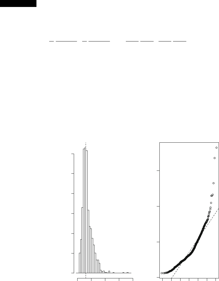
nonnormality.

SD ratio

Density

0 5 10 15 20

−3 −2 −1

Quantiles of Standard Normal

SD ratio

0.30

0.25

0.20

0.15

0.10

0.05

0.00

Figure 10.13 Histogram and normal plot of bootstrap standard deviation ratios from R

10.6 Comparisons Using the Bootstrap and Permutation Methods 537