Dorst L., Fontijne D., Mann S. Geometric Algebra for Computer Science. An Object Oriented Approach to Geometry
Подождите немного. Документ загружается.

342 APPLICATIONS OF THE HOMOGENEOUS MODEL CHAPTER 12
R
A
[x
A
]
R
B
[x
B
]
A
a
x
B
b
e
o
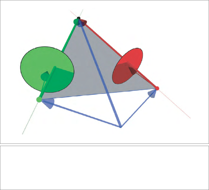
Figure 12.3: The epipolar constraint. We show two cameras A (in red) and B (in green) with
their observations of the same point X. In the world, these give the vectors R
A
[x
A
] from the
location a of camera A and R
B
[x
B
] from the location b of camera B. Since the cameras are
looking at the same point, these ray vectors must be in one plane with the relative position
vector b − a, and that is the epipolar condition. For clarity in visualization, we have followed the
habit of most literature to draw the image planes in front of the pinholes.
In the classical treatment of the epipolar constraint, there are of course no trivector
equations. We get to a scalar equation by taking the Euclidean dual of (12.13), which
gives
0 = x
A
· (t
A
× R
B
A
[x
B
]).
This is the form in which you find the epipolar constraint in texts on stereo vision,
although it is often formulated in matrix form
0 = [[ x
A
]]
T
[[ t
×
A
]] [[ R
B
A
]] [[ x
B
]]
by introducing the matrix [[ t
×
A
]] that performs the cross product with t
A
. The combination
[[ E
B
A
]] = [[ t
×
A
]] [[ R
B
A
]] is known as the essential matrix of the stereo vision problem.
12.2.4 LINE-BASED STEREO VISION
In more advanced stereo vision, one does not use only potential point matches to recon-
struct the depth image of reality, but also line matches. In the usual formulation, the
SECTION 12.2 IMAGING BY MULTIPLE CAMERAS 343
representation of such lines and the matches that are their consequences is not always
straightforward. The reason is that you require Pl
¨
ucker coordinates to represent lines, and
this is an extra representational step in the classical approaches. In the geometric algebra
approach, lines are natural elements of the algebra, just like points are, and the formu-
lation of the line-based stereo matching is more clearly analogous to that for points. We
investigate that briefly in this section.
Consider a camera A as above, with rigid body motion A[·], but now look at the inter-
pretation of an observed line in the image plane. First, place a camera in the origin, in
standard orientation. A line in the image plane at location x
in the image and direction u
(parallel to the image plane) is
L = (e
0
+ f + x) ∧ u = e
0
u + M,
so it is characterized by a direction vector u
and a 3-D moment 2-blade M = (f + x) ∧ u.
This line generates the plane of rays from the pinhole e
0
:
e
0
∧ L = e
0
∧ M,
(12.14)
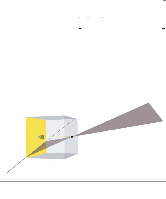
which only depends on the moment of the line; see Figure 12.4. The 3-D Euclidean
2-blade M thus completely characterizes the observed line (obviously, you can retrieve
the direction by intersection with the image plane), and we will denote the observed line
by this 2-blade. (This is also shown by the matr ix of the line projection in (12.11), which
only involves the coordinates of the moment.) Note the subtle difference between the
f
M
e
0
L
Figure 12.4: The plane of rays generated by a line observation L is characterized by its
moment 2-blade M.
344 APPLICATIONS OF THE HOMOGENEOUS MODEL CHAPTER 12
effectively observed line M and the real-world 3-D line L, and how (12.14) expresses that
they are geometrically and algebraically identical when seen from the pinhole.
Moving the camera to its general position and orientation by its rigid body motion A,we
find that an observed line L
A
in the image corresponds to a potential plane
A[e
0
∧ L
A
] = A[e
0
∧ M
A
] = (e
0
+ a) ∧ R
A
[M
A
].
Now consider three cameras A, B, C, each observing the same line L as L
A
, L
B
, and L
C
,
respectively, in their own local frames of reference. The world planes of the observed lines
should intersect in line L. Algebraically, we can express this by stating that their
meet
naïvely computed with the pseudoscalar e
0
I
3
as a join is zero (since they are not in gen-
eral position). This gives the equation
0 = (A[e
0
∧ L
A
])
∗
∧ (B[e
0
∧ L
B
])
∗
∧ (C[e
0
∧ L
C
])
∗
.
To get more specific in the consequences, we expand the rigid body motion in its trans-
lational and rotational parts and write the full dual in terms of the Euclidean dual (since
I
4
= e
0
I
3
,wehaveX
∗
= X
夹
e
−1
0
). As shorthand, we define Euclidean dual moment vec-
tors m
A
≡ M
A
夹
, and so on, in local camera coordinates, and their rotated versions m
A
,
m
B
, m
C
to world coordinates:
m
A
≡ R
A
[m
A
] = R
A
[M
A
]
夹
,
m
B
≡ R
B
[m
B
] = R
B
[M
B
]
夹
,
m
C
≡ R
C
[m
C
] = R
C
[M
C
]
夹
.
The m
A
, m
B
, m
C
are dual representations of the planes of the rays for each of the lines and
therefore simply dual representations of the observed lines in all their projective essence.
You may think of them as the observed lines. The m
A
, and so on, are those directions
transferred to world coordinates. Then we obtain
0 =
(e
0
+ a) ∧ R
A
[M
A
]
∗
∧
(e
0
+ b) ∧ R
B
[M
B
]
∗
∧
(e
0
+ c) ∧ R
C
[M
C
]
∗
= ((e
0
+ a)( m
A
e
−1
0
)) ∧ ((e
0
+ b)( m
B
e
−1
0
)) ∧ ((e
0
+ c)( m
C
e
−1
0
))
=
(a · m
A
) e
−1
0
− m
A
∧
(b · m
B
) e
−1
0
− m
B
∧
(c · m
C
) e
−1
0
− m
C
= −m
A
∧ m
B
∧ m
C
+
(a · m
A
) ∧ m
B
∧ m
C
− m
A
∧ (b · m
B
) ∧ m
C
+ m
A
∧ m
B
∧ (c · m
C
)
e
−1
0
.
Therefore, there are two equations that follow from the triviality of the
meet:
0 = m
A
∧ m
B
∧ m
C
and
0 = (a · m
A
) m
B
∧ m
C
− (b · m
B
) m
A
∧ m
C
+ (c · m
C
) m
A
∧ m
B
.
The first equation has a simple geometrical interpretation: the m
i
are the normal vectors
of planes through a common line L, and these are of course coplanar. The second involves
the positional aspects, and is more quantitative.

SECTION 12.2 IMAGING BY MULTIPLE CAMERAS 345
We can interpret these equations as a condition on any of the observed lines, given the
other two lines. Let us develop this for m
A
.Tofactorizem
A
out of the second equation
(in terms of the outer product), we need to get rid of the first term. We can do so by taking
the inner product with a of the first equation, which gives
0 = (a · m
A
) ∧ m
B
∧ m
C
− (a · m
B
) ∧ m
A
∧ m
C
+ (a · m
C
)m
A
∧ m
B
.
Inserting this into the second equation yields
0 = m
A
∧
(c − a) · m
C
m
B
−
(b − a) · m
B
m
C
. (12.15)
Given the observed lines m
B
and m
C
in their local coordinates, plus the relative poses
of the cameras as given by A, B, C, this specifies what m
A
should be (modulo the usual
homogeneous scale factor). This is a linear relationship of two variables m
B
and m
C
to
provide a third: it is a tensor, and we can rewrite it symbolically as a mapping T w ith two
arguments:
0 = m
A
∧ T(m
B
, m
C
).
T is called the trifocal tensor. One can derive similar trifocal tensors by factoring out m
B
or m
C
, so there are three of them in this situation.
Converting this into the more classical coordinate form, we consider everything relative
to camera A. This means that we should apply A
−1
to the tensor equation. All elements
involved are Euclidean direction elements, so they simply transform by R
−1
A
. Let us abbre-
viate R
B
A
≡ R
−1
A
R
B
and R
C
A
≡ R
−1
A
R
C
, and the relative position of the cameras B and C in
terms of A as t
B
≡ R
−1
A
[b − a] and t
C
≡ R
−1
A
[c − a].
2
0 = m
A
∧
R
B
A
[m
B
](t
C
· R
C
A
[m
C
]) − (R
B
A
[m
B
] · t
B
) R
C
A
[m
C
]
The result is then written in terms of matrix operations on vectors (since that is all you
have classically), or in tensor notation. The i
th
coordinate of the line m
A
is proportional to
[[ m
A
]]
i
∝ [[ m
B
]]
j
[[ R
B
A
]]
j
i
[[ t
C
]]
l
[[ R
C
A
]]
k
l
− [[ R
B
A
]]
j
m
[[ t
B
]]
m
[[ R
C
A
]]
k
i
[[ m
C
]]
k
= [[ T]]
jk
i
[[ m
B
]]
j
[[ m
C
]]
k
,
so that gives the trifocal tensor in tensorial notation (including the usual summation con-
vention over repeated upper and lower index pairs).
2 In the other literature on multicamera treatments, it is customary to parameterize the rigid body motion inversely
(not where the camera frame is in the world frame, but vice versa). Replace our rotations like
R with R
−1
and t
with −R
−1
t to get that parameterization. It simplifies the appearance of the final results somewhat, since an R
gets absorbed into the new t twice.
346 APPLICATIONS OF THE HOMOGENEOUS MODEL CHAPTER 12
The trifocal constraint of (12.15) can be used to derive constraints on points as well as
lines. For example, if we know the two observed lines m
B
and m
C
, and wonder what the
constraint might be for a point x
A
to be the projection of the line Λ, then this follows
immediately from the demand that it should lie on the line L
A
,whichisx
A
∧ e
0
∧ M
A
= 0,
so x
A
∧ M
A
= 0. Introducing x
A
= A[x
A
] = a + R
A
[x
A
] as the same point in world
coordinates, we have x
A
· m
A
= 0, so that the constraint on the point is obtained by
taking the inner product of the trifocal constraint with x
A
:
0 = (x
A
· m
B
)
(c − a) · m
C
−
m
B
· (b − a)
(x
A
· m
C
).
Therefore, x
A
lies on the dual line
m
B
(c − a) · m
C
−
m
B
· (b − a)
m
C
.
Another way of looking at the trifocal tensor is as a line-parameterized homography (i.e., a
a projective mapping between spaces). Suppose we fix m
C
; then this determines a spatial
plane, which can be used to transfer points in B that are observations from the same world
line to points in A (project the ray of observation x
B
to meet the plane in a point, then
observe this point as x
A
). This mapping can be extended uniquely to the whole image
plane as a homography. We can give an explicit formula for this homography between the
planes A and B: it should be proportional to the inverse adjoint of the mapping for lines
m
A
and m
B
,givenm
C
. T he adjoint of
m →
(c − a) · m
C
R
B
[m] −
(b − a) · R
B
[m]
m
C
is easily found as
x →
(c − a) · m
C
R
−1
B
[x] − (m
C
· x) R
−1
B
[b − a],
and we take the inverse by simply considering this not as a mapping from x
B
to x
A
, but
from x
A
to x
B
. Therefore the homography between image A and image B is
x
B
∝
(c − a) · m
C
R
A
B
[x
A
] − (m
C
· x
A
) R
A
B
[b − a].
Similarly, you can derive where a point should be in image A once you have observed it
in image B and C, just using the trifocal tensor.
If you therefore have a robotic environment in which you see enough lines for which you
are able to do the correspondence in the three images, then you can estimate the trifocal
tensor (using techniques from [25]), and employ this to compute other correspondences
between the images as well.
12.3 FURTHER READING
The impressive book by Faugeras and Luong [21] deals with the geometry of mul-
tiple cameras. Like [60], it uses the Grassmann-Cayley algebra of the outer product
SECTION 12.4 EXERCISES 347
(which they call join) and its adjoint (which they call meet). This provides a concept
of duality, but no metric. The book contains a compact mathematical explanation of
this structure, illustrated with geometrical usage. Unfortunately, the authors quickly
revert to a matrix-based notation in the chapters that put the str ucture to practical use,
and what could have been explicitly defined algebraic products become tricks in matrix
manipulation.
Another modern reference on the geometry of imaging is [25], which dextrously
avoids using even Grassmann algebra. All operations are expressed in terms of matrices
or tensors defined in terms of Pl
¨
ucker coordinates. The powerful results can therefore
be implemented directly, but the geometrical structure of the techniques is often hard
to grasp.
We find that both these books have become much more accessible now that geometric
algebra offers a structural, representation-independent insight to help one understand
what is essentially going on. They can then be browsed quickly for useful techniques.
12.4 EXERCISES
12.4.1 STRUCTURAL EXERCISES
1. Table 12.1 contains the case in which a line {a, m} is extended to a plane by
an additional direction n to form the plane [a × n : n · m]. Demonstrate the
correctness of this formula by representing the spanning L ∧ n in terms of the
Pl
¨
ucker coordinates.
2. Show that the solution of x from the relationship e
0
∧ x = e
0
∧ x of (12.7) is indeed
x = e
−1
0
(e
0
∧ x), and understand to your satisfaction that this still gives the cor-
rect vector x for the point x, even when the latter would have been given relative to
another origin e
0
for the homogeneous coordinates.
3. Knowing some of the standard formulas in geometric algebra, you may recognize
that the central projection formula (12.9) is not unlike the usual orthogonal pro-
jection formula onto a line with direction a, which maps x to (x · a) a
−1
. Demon-
strate that we can consider the central projection x
→ x /( f
−1
· x) as the fixed
vector f gets inverted, projected onto the variable vector x, and then reinverted, to pro-
duce x
. This interpretation of the formula generalizes to substituting x by a line
or plane (just replace the inner product with the contraction); it then produces
the support vector of the projected line or plane. (Hint: Show that x
satisfies:
x
−1
= (f
−1
· x) x
−1
= (f
−1
· x
−1
) x and interpret.)
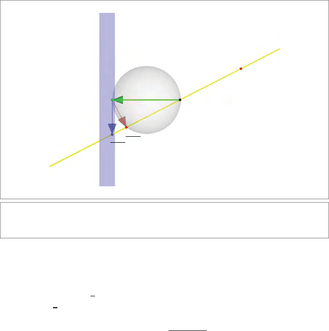
4. Show that the images of all x under the construction of the previous exercise before
the final inversion (that is, (f
−1
· x)/x) lie on a sphere through the pinhole and
the end of the vector f
−1
. This is sketched in Figure 12.5 for f = |f = 1.Itbears
uncanny resemblance to an eyeball!
348 APPLICATIONS OF THE HOMOGENEOUS MODEL CHAPTER 12
f
f
x
f
−1.
x
x
x
f
−1.
x
o
Figure12.5: The projection of the optical center f onto all rays through the pinhole generates
an eyeball.
5. Equation (12.9) gives the projection of a unit 3-D point at location x to become a
point at location x
, which is on the image plane, but it is not expressed yet in image
plane coordinates x
. Show that the mapping from the 3-D point at x to the image
point at x
= x
− f can be written as
x →
f (f
−1
∧ x)
f
−1
· x
.
Interpret this expression geometrically, especially the numerator.
6. Represent the result of the previous problem in homogeneous coordinates, using
the center of the image at f as origin. Before you do so, guess the answer!
12.5 PROGRAMMING EXAMPLES AND EXERCISES
12.5.1 LOADING TRANSFORMATIONS INTO OPENGL
This example illustrates the good interoperability between homogeneous coordinates-
based software (such as OpenGL) and the homogeneous model.
Any outermorphism can be straightforwardly loaded into OpenGL. First, the images
of the four basis vectors under the outermorphism are computed, and then the matrix
SECTION 12.5 PROGRAMMING EXAMPLES AND EXERCISES 349
representation of the outermorphism is constructed, whose coordinates are then loaded
onto the modelview mat rix of OpenGL.
We use a translation-rotation as an simple example. In our OpenGL examples so far,
loading this transformation to the modelview matrix would be implemented as:
glTranslatef(0.0f, 0.0f, distance); // translate
rotor R = g_modelRotor;
rotorGLMult(R); // rotate (implemented in h3ga_util.cpp)
Using the matrix representation of the outermorphism, this becomes:
// get the translation vector & the rotor
h3ga::vector T = _vector(distance * e3);
rotor R = g_modelRotor;
rotor Ri = _rotor(inverse(R));
// compute images of basis vectors:
point imageOfE1 = _point(R * e1 * Ri + (T ^ (e0 << (R * e1 * Ri))));
point imageOfE2 = _point(R * e2 * Ri + (T ^ (e0 << (R * e2 * Ri))));
point imageOfE3 = _point(R * e3 * Ri + (T ^ (e0 << (R * e3 * Ri))));
point imageOfE0 = _point(R * e0 * Ri + (T ^ (e0 << (R * e0 * Ri))));
// create matrix representation:
omPoint M(imageOfE1, imageOfE2, imageOfE3, imageOfE0);
// load matrix representation into GL modelview matrix:
glLoadMatrixf(M.m_c);
For this simple example, it is of course counterproductive to replace the short OpenGL
code with its geometric algebra equivalent: the example is intended to demonstrate the
principles only.
12.5.2 TRANSFORMING PRIMITIVES WITH OPENGL MATRICES
This example performs the opposite of the previous example. Instead of setting the
OpenGL modelview matrix using the matrix representation of an outermorphism, it
reads out the modelview matrix and turns it into a matrix representation of an outer-
morphism. The actions are as follows:
•
The code reads the OpenGL transformation matrix;
•
It loads this into a matrix representation of an outermorphism;
•
It resets the OpenGL modelview matrix;
•
It applies the transform to the primitives, and then draws them.
We can then transform not only points, but also lines and planes, as this example is just
the example from Section 11.13.2 with some modifications.
350 APPLICATIONS OF THE HOMOGENEOUS MODEL CHAPTER 12
To initialize the matrix representation of the outermorphism, we use:
// extract OpenGL modelview matrix
float MVM[16];
glMatrixMode(GL_MODELVIEW);
glGetFloatv(GL_MODELVIEW_MATRIX, MVM);
// reset OpenGL modelview matrix (we will apply the transform ourselves)
glLoadIdentity();
// initialize the images of the basis vectors:
point images[4];
for (int i=0;i<4;i++) {
images[i].set(point_e1_e2_e3_e0, &(MVM[i * 4]));
/* or:
images[i].set(point_e1_e2_e3_e0,
MVM[i*4+0],
MVM[i*4+1],
MVM[i*4+2],
MVM[i*4+3]);
*/
}
// initialized matrix representation of outer morphism
om M(images);
To draw any primitive (point, lines, plane):
void applyTransformAndDraw(const om &M, const mv &X) {
// apply the outermorphism:
mv MX = apply_om(M, X);
draw(MX);
}
The actual code is slightly more complicated due to the use of a custom probing point;
see the GA sandbox source code package.
In the graphics, there is a somewhat undesirable side effect due to the explicit use of a basis
in a factorization algorithm that is used to draw the plane. It is best observed by starting
the example and rotating the scene (drag the left mouse button along the edges of the
viewport). You will notice that edges of the depicted plane stay in place while the rest of
the scene rotates. This feels counterintuitive (compare this to Example 11.13.2 where the
edges do rotate).
The cause of this is the following. To draw the plane, we need two vectors that span it. We
obtain these by factorization, using the (basis-dependent) algorithm described in Sec-
tion 21.6. In the original example (Section 11.13.2), we factor the plane, transform the
factors, and then draw the plane using the rotated factors. Then the plane rotates visibly,
because its vector factors do. In the present example, we first rotate the plane, then factor
it, and then draw the rotated plane using its factors. When the rotation plane is the same

SECTION 12.5 PROGRAMMING EXAMPLES AND EXERCISES 351
as the plane itself, the rendering of the plane will not change at all. Intuitively, the former
is better, but algebraically, the latter result is more correct, for it shows the true behavior
of a plane under rotation.
12.5.3 MARKER RECONSTRUCTION IN OPTICAL MOTION
CAPTURE
In Section 10.7.3 we implemented an algorithm for external camera calibration. That
algorithm computed the position and orientation of any number of cameras. The cur-
rent example builds upon that earlier example by using the calibrated cameras to perform
measurements of the position of markers. We use the homogeneous model to reconstruct
3-D markers from actual capture data. Figure 12.6 shows the example in action.
The markers are little spheres (size from 0.5–3.0 cm) wrapped in retroreflective tape. Every
time the camera records an image (between 20 to 500 times per second), an LED ring
around the camera lens illuminates the scene, and the markers reflect this light back to
the camera sensor. With proper exposure time (our system typically uses between 0.2 and
1ms), the result is that the markers are visible as bright blobs in the otherwise black images.
The centers of the 2-D markers are easily retrieved from the images, since the center of
a projected sphere is a good approximation to the projection of the center of that sphere
when the markers are sufficiently far away.
When a marker is visible from multiple calibrated camer as, its position can be recon-
structed by computing the intersection point of rays from the camera centers through
Figure 12.6: Example 3 in action. The four red arrows are the cameras and the black dots
are the reconstructed markers. When the example is in motion, it is immediately clear that the
black dots are attached to a human.