Dorst L., Fontijne D., Mann S. Geometric Algebra for Computer Science. An Object Oriented Approach to Geometry

Подождите немного. Документ загружается.

352 APPLICATIONS OF THE HOMOGENEOUS MODEL CHAPTER 12

Marker

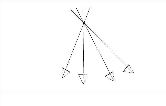
Image plane

Camera pinhole

Figure 12.7: Reconstruction of markers.

the marker center. This is illustrated in 2-D in Figure 12.7. Markers can of course be

occluded by the subject to which they are attached, so not all cameras can see every marker

all the time. The more cameras that actually see a particular marker, the more precise

the reconstruction can be. The simplistic marker reconstruction algorithm used in this

example reconstructs the markers as follows: we iterate over every pair of 2-D markers

from two different cameras. For each pair, we perform the following actions:

•

First, we construct a plane through the two camera centers and the 2-D marker in

the image plane of one camera. This plane is then intersected with the image plane

of the other camera to compute the epipolar line:

// normalizedPoints P1, P2 are the camera positions.

// normalizedPoint M1 is the marker position, on image plane of

// camera 1.

// plane IP2 is the image plane of camera 2.

// compute the epipolar line in the image plane of camera 2:

line L2 = _line(unit_r(dual(P1 ^ M1 ^ P2) << IP2));

•

Once we have the epipolar line, we search for 2-D markers sufﬁciently close to it (as

the data is inherently noisy, we will rarely have a precise intersection of the epipolar

line with a marker). We compute the distance of each candidate marker as (

M2*)L2:

// normalizedPoint M2 is the marker position, on image plane of

// camera 2

SECTION 12.5 PROGRAMMING EXAMPLES AND EXERCISES 353

// compute distance in image plane:

mv::Float distance = fabs(_Float((M2 << IP2) << L2));

The dual is of course taken relative to the image plane of the second camera.

•

If the distance is less than some epsilon value, we reconstruct a 3-D marker by

computing the average of the closest points on the two lines

P1 ∧ M1 and P2 ∧ M2.

We collect all reconstructed points in an array. How these points are computed is

described below.

After this loop, we iterate over all pairs of reconstructed 3-D markers to ﬁnd the ones that

are sufﬁciently close in 3-D space (where close is typically deﬁned as within the distance

of the radius of the marker). We merge close markers by summing them. We do not nor-

malize the points, as we use the

e0 coordinates as a rough counters for how many cameras

contributed to a particular reconstruction. We return only those markers that have been

seen by a sufﬁcient number of cameras:

R is the array of reconstructed 3D markers (candidates).

‘reconstructedMarkers’ is the final array of 3D markers

(normalizedPoints) that is returned to the caller.

if ((int)R[i].e0() >= minNbCameras) {

reconstructedMarkers.push_back(_normalizedPoint(R[i] /

R[i].e0()));

}

When you read the full source code of the example in the GA sandbox source code pack-

age, you may encounter some use of the conformal model of the later chapters. Our actual

motion capture system is based primarily on the conformal model, hence this example

(which was derived from it to illustrate homogeneous model techniques) stores the cam-

era transformations as conformal versors.

A more reﬁned reconstruction algorithm would use some kind of data structure to quickly

look up points close to particular epipolar lines. For each successful match in two cam-

eras, an initial 3-D marker is then reconstructed. These 3-D markers can subsequently be

projected onto the image planes of the other cameras, after which another data structure

(e.g., a spatial hashing table) can be used to quickly ﬁnd markers in the v icinity of the

projected points. A least-squares-based solution (see Section 10.4.2) would then be used

to ﬁnd the optimal reconstruction of the 3-D marker given the 2-D measurements in each

camera.

Computing Closest Points on Lines

Computing the closest points on two skew lines is an important operation that is

performed in the inner loop of by the reconstruction algorithm. We provide an efﬁcient

geometric algebra implementation in Figure 12.8. The two lines are passed in factored

form (i.e., as points and directions such that the actual lines are

P1∧D1 and P2∧D2).

354 APPLICATIONS OF THE HOMOGENEOUS MODEL CHAPTER 12

bool closestPointsOnCrossingLines(

const normalizedPoint &P1, const h3ga::vector &D1,

const normalizedPoint &P2, const h3ga::vector &D2,

mv::Float &d1, mv::Float &d2) {

// Compute difference between starting points

h3ga::vector dif = _vector(P2 - P1);

// compute inverse pseudoscalar of space spanned by D1 and D2

bivector I = _bivector(D1 ^ D2);

if (_Float(norm_e2(I)) == 0.0f) // check parallel

return true; // returning true means ’lines are parallel’

bivector Ii = _bivector(inverse(I));

// compute reciprocals:

h3ga::vector rD1 = _vector(D2 << Ii);

h3ga::vector rD2 = _vector(D1 << Ii);

// solution:

d1 = _Float(rD1 << dif);

d2 = _Float(rD2 << dif);

return false;

}

Figure 12.8: Crossing lines code.

The function returns scalars d1 and d2 such that P1+d1∗ D1 and P2+d2∗ D2 are

the closest points on the two lines.

The function works by projecting the vector

P2—P1 onto the bivector D1∧D2. The geo-

metric intuition behind this is that we are trying to minimize the distance

P2—P1between

the two points by moving along the lines.

d1 and d2 are the coordinates of the projected

vector relative to the basis spanned by

D1 and D2. Because D1 and D2 are not orthonormal,

we need to compute their reciprocals (

rD1 and rD2) ﬁrst.

THE CONFORMAL MODEL:

OPERATIONAL EUCLIDEAN

GEOMETRY

In the previous chapters, we studied the geometric algebra version of the homogeneous

model. The homogeneous model of Euclidean geometry is reasonably effective since it lin-

earizes Euclidean transformations, and geometric algebra extends the classical homoge-

neous coordinate techniques nicely through its outermorphisms. However, we remarked

that we were not able to use the full metric products of geometric algebra, since the met-

ric of the model was only indirectly related to the metric of the Euclidean space we had

wanted to model.

Fortunately, we can do better. In the next few chapters, we present the new conformal

model for Euclidean geometry, which can represent Euclidean transformations as orthog-

onal t ransformations. Encoding those as versors, we get the full power of geometric alge-

bra, including the structure preservation of all constructions.

In this chapter, we start the exposition by deﬁning the new representational space (which

has two extra dimensions and an indeﬁnite metric) and showing what its vectors repre-

sent. The two extra dimensions are geometrically interpretable as the point at the orig in

(as in the homogeneous model) and the point at inﬁnit y (which nicely closes Euclidean

geometry, making translations into rotations around inﬁnity).

We then focus on how to represent the familiar ﬂats and directions already present in the

homogeneous model and how to move them around. As ﬁrst applications, we use the

355

356 THE CONFORMAL MODEL: OPERATIONAL EUCLIDEAN GEOMETRY CHAPTER 13

versor representation to provide straightforward closed-form interpolation of rigid body

motions and universally valid constructions for the reﬂection of arbitrary elements.

The natural coordinate-free speciﬁcation of elements and operations in the conformal

model is best appreciated using the interactive illustrations. Even more than in the pre-

vious chapters, we encourage you to play around with the interactive software provided

with this book.

13.1 THE CONFORMAL MODEL

The conformal model is especially designed for Euclidean geometry, which is the

geometry of transformations preserving the Euclidean distances of and within objects.

These Euclidean transformations are sometimes called isometries, and they include trans-

lations, rotations, reﬂections, and their compositions.

We will occasionally limit ourselves to Euclidean motions, which are the Euclidean trans-

formations that can be performed a little at a time. These are also known as rigid body

motions, and they consist of compositions of translations and rotations. They are proper

isometries, i.e., they preserve the Euclidean distances and handedness.

To emphasize that the conformal model involves the representation of Euclidean

geometry, we will denote the base space by

rather than R

n,0

. This notation is meant

to suggest that the group of Euclidean transformations is to be represented in the model

as well.

13.1.1 REPRESENTATIONAL SPACE AND METRIC

We start with some observations on points in a Euclidean space.

•

A Euclidean space E

has points at a well-deﬁned distance from each other. If two

points P and Q were created by a translation over the Euclidean direction vectors p

and q from some origin O, then their squared distance is d

(P, Q) = p − q

(p − q) · (p − q ). In many respects, these squared distances are more convenient

to compute with than the actual distances; for instance, Pythagoras’ theorem states

that squared distances can be added under certain conditions.

•

Euclidean spaces do not really have an origin: there is no special ﬁnite point that can

be distinguished from other points. If an origin is used, it is for convenience, as a

point to relate other points to. Similarly, there are no preferential directions, though

it may be convenient to deﬁne an arbitrary standard frame at the equally arbitrary

origin.

•

Mathematicians have long known that it is convenient to close a Euclidean space

by augmenting it with a point at inﬁnity. (They call this compactiﬁcation.) That

point at inﬁnity is a point in common to all lines and planes, and invariant under

SECTION 13.1 THE CONFORMAL MODEL 357

the Euclidean transformations. Having it explicit makes the algebraic patterns in

geometrical statement more universal.

When constructing a model for Euclidean geometry, we take these properties as central.

The arbitrariness of the origin was something we wanted in the homogeneous model, and

it was partly achieved by assigning an extra dimension to it in a representational space. So

we need at least need an (n+1)-dimensional representational space. We are now also going

to assign an extra dimension to the special point at inﬁnity. In our model, we represent it

as a vector denoted as ∞, to remind us of what it is. (There will be no confusion with the

number inﬁnity.) This turns our representational space for the n-dimensional Euclidean

space

from (n + 1)-dimensional to (n + 2)-dimensional.

The interface between geometry and algebraic representation is that we represent Euclidean

points in

by representative vectors in the (n + 2)-dimensional representational vector

space. The inﬁnite point is represented by the vector ∞. A ﬁnite point P is represented by

avectorp, with certain additional properties that we specify below. Now we still have the

freedom to choose the metric of this representational space (and we must specify it if we

want to endow it with a geometric algebra). We use this metric to encode the Euclidean

distance in

. In view of the observed linear behavior of square distances we do so as

follows:

p · q ∼ d

(P, Q).

(13.1)

On the left you see the inner product of two vectors of the representational space; on

the right you see the squared distance of two points in the Euclidean space

.Theyare

directly proportional! (There are some scaling factors that we introduce below for back-

wards compatibility, but those are irrelevant to the principle of the setup.)

One immediate consequence of this deﬁnition of the metric is that a vector p representing

a ﬁnite point must obey p · p = 0, since the Euclidean distance of a point to itself is

zero: d

(P, P) = 0. Therefore, Euclidean points are represented by null vectors in the

representational model. A null vector is a vector with norm zero; in a Euclidean space,

such a vector would have to be the zero vector, and we could not use that to denote a

great variety of points. So the (n + 2)-dimensional representational space must be non-

Euclidean.

Null vectors may seem strange, but it is fairly easy to make them in a manner that feels

only moderately irregular. We may alternatively construct the (n + 2)-dimensional rep-

resentational space by augmenting the regular n Euclidean dimensions with two special

dimensions, for which a basis is formed by two vectors e and

e that square to +1 and −1,

respectively, and that are orthogonal (so that e·

e = 0). Having these, it is easy to make null

1 The homogeneous model has location-independent directions, which we identiﬁed as being characterized by

improper points on the heavenly sphere, but this has a different ﬂavor than a single point at inﬁnity, which is a

location that one can approach from

any direction. We will not lose those extra elements representing directions

for they are also found as elements in the new model.

358 THE CONFORMAL MODEL: OPERATIONAL EUCLIDEAN GEOMETRY CHAPTER 13

vectors out of them: the vectors (e +

e) and (

e − e) are both null without being zero, as you

can check easily by squaring them. In this construction, the representational space has an

orthonormal basis consisting of (n + 1) positive dimensions (with basis vectors squaring

to +1) and 1 negative dimension (with basis vector squaring to −1). We therefore denote

it by

n+1,1

. Such a space is called a Minkowski space in physics, where it has been well

studied to represent space-time in relativity; the negative dimension is then employed

to represent time. We will ﬁnd a geometrically more natural basis than e and

e for the

conformal model, but the representational space is still the metric space

n+1,1

This (n + 2)-dimensional space requires n + 2 coefﬁcients to specify a vector. We should

require only n coefﬁcients to specify a point in Euclidean space, so there is more in this

space than we appear to need. Since points are represented by null vectors, their repre-

sentatives must obey p · p = 0, and this is a condition on their coefﬁcients that removes

onedegreeoffreedom,leavingn + 1. The remaining degree of freedom we use to denote

the weight of the point, as in the homogeneous model. In that model, we retrieved the

weight as e

−1

· p, since it was the coefﬁcient of e

; in the present model we extract it by

the operation −∞ · p. The relationship of inner product to distance of (13.1) should of

course be deﬁned on properly normalized points, since it is independent of the weight,

so in that formula we should divide p by its weight, and q as well. We introduce an extra

scaling factor of −

for convenience later on, and actually deﬁne the inner product of

vectors representing points through

−∞ · p

−∞ · q

≡−

(P, Q). (13.2)

(The two minus signs on the left of course cancel each other, but we would like to get you

used to viewing −∞ · p as a weight-computing expression.) Equation (13.2) is in fact the

deﬁnition of the representational model; all the rest of the correspondence between ele-

ments of its geometric algebra and Euclidean geometry follows from it without additional

assumptions.

The model thus constructed was called the conformal model in the literature, for the

mathematical reason that it is capable of representing conformal transformations by ver-

sors. We will demonstrate that in Chapter 16, but prefer to focus on its use for Euclidean

transformations ﬁrst. We will show that it is an operational model for Euclidean geom-

etry in the double sense that Euclidean transformations are represented as structure-

preserving operators, which are moreover easy to put to operational use. In view of that,

we would prefer to call it the operational model for Euclidean computations. This is too

much of a mouthful, so we might as well conform to the term conformal model, despite

its arcane origins.

Even though the conformal model hit computer science only a few years ago, when it was

introduced by Hestenes et al. in 1999 [31], we are beginning to ﬁnd that we could have had

the pleasure of its use all along. Considerable elements of it are found in much older work,

and it appears to have been reinvented several times. We do not know the whole story yet,

SECTION 13.1 THE CONFORMAL MODEL 359

but markers on the way are Wachter (a student of Gauss), Cox [9] and Forder 1941 [22]

(who used Grassmann algebra to treat circles and their properties), Angl

es 1980 [2] (who

showed the crucial versor form of the conformal transformations) and Hestenes (who

had already presented it in his 1984 book [33] but only later realized its true importance

for Euclidean geometry). We are convinced that its time of general adaptation has ﬁnally

arrived, since the conformal model is much more clearly useful to actually programming

geometrical applications than it is to theorizing about geometry on paper.

13.1.2 POINTS AS NULL VECTORS

Let us be more precise about the point representation. As we realized before, the relation-

ship of the metric to the Euclidean distance implies that ﬁnite points are represented by

null vectors. What about the point at inﬁnity?

The point at inﬁnity is represented by ∞, and it should have inﬁnite distance to all ﬁnite

points. Substituting q = ∞ in (13.2), we ﬁnd that an inﬁnite result is reached only if we

set ∞·∞= 0. This implies that the point at inﬁnity is also represented by a null vector.

Null vectors in the conformal model

n+1,1

represent Euclidean points of E

(both ﬁnite and inﬁnite).

After you have gotten used to this correspondence, it becomes natural to identify repre-

sentative null vectors with points and talk about the null vector p as “the point p” rather

than as “representing the point P.” We will gradually slip into that convenient usage as

this chapter evolves.

We call a point p normalized or a unit point when its weight equals 1:

−∞ · p = 1

We may be tempted to select one special unit point O as the origin of our space and

represent it by a vector denoted o. It would then be a special vector in the conformal

model with the property o ·∞ = −1,aswellaso · o = 0, by virtue of being a point. It

therefore appears to bear a special relationship to the vector ∞ representing the point

at inﬁnity: though both are null vectors, they are (minus) each other’s reciprocals in

the sense that o ·∞ = −1. That simpliﬁes the math of computing with them, and it

reveals that the weight of a point is the coefﬁcient of o of its representative vector (for a

coefﬁcient of a vector is retrieved by an inner product with its reciprocal, as we saw in

Section 3.8—so the o coefﬁcient is retrieved by an inner product with −∞). The strong

parallel with e

and e

−1

in the homogeneous model suggests that an arbitrary unit point

might be writable as o + p, but this is not a null vector (it squares to p

). We should

use the extr a dimension to represent a unit point as p = o + p + α ∞, with an α that

should be determined by the null vector condition p · p = 0. You can easily verify that

this gives

360 THE CONFORMAL MODEL: OPERATIONAL EUCLIDEAN GEOMETRY CHAPTER 13

p = o + p +

∞ (13.3)

as the representative null vector for a unit point relative to the origin o.

Equation (13.3) resembles a coordinate representation of the vector p in terms of a purely

Euclidean location vector p and two extra terms in a {o, ∞}-basis for the extra two dimen-

sions of the conformal model. It is somewhat misleading: although ∞ indeed has special

signiﬁcance, the origin point o does not. Any unit point could have been used as origin; it

would have had the same relationships with ∞ (since any ﬁnite point p obeys −∞·p = 1),

and would merely have changed the value of the location vector p for the particular point

P we are considering. So (13.3) is deceptive in that it is too speciﬁc. Still, it is convenient

to have, since it gives a connection to the homogeneous representation (o is like e

), and

even to the vector space model (in exhibiting the Euclidean location vector p). You can

use it when you begin to work with the conformal model—as you advance, you will dare

to work coordinate-free, merely using the algebraic properties of the point p, and that will

make your formulas and algorithms more generally applicable.

But while we have this speciﬁc representation, let us use it to verify the consistency with

the original deﬁnition of the metric:

p · q = (o + p +

∞) · (o + q +

∞)

= −

+ p · q −

= −

(q − p)

. (13.4)

Note how the metric of the conformal model plays precisely the r ight role to compose the

correct terms in the squared difference required to express the Euclidean distance. So the

conformal model indeed does what it was designed to do.

Letting p become large in (13.3), the dominant term is proportional to +∞. This shows

the reason for our choosing the normalization such that ∞·p is negative: now +∞ is

positively proportional to (the vector representing) the point at inﬁnity.

We are especially interested in the Euclidean space

, and when required, we use an

orthonormal basis {e

} for that part of the representation. That leaves the other

two elements in the basis of

n+1,1

. Earlier, we brieﬂy introduced the basis {e,

e} with

their squares of +1 and −1, and that would work as basis for the part

1,1

. But it is often

geometrically more signiﬁcant to make a change of basis to the two null vectors o and

∞, representing our arbitrary origin and the point at inﬁnity. These null vectors can be

deﬁned in terms of e and

e as

2 We should mention that the standards in this new model have not quite been established yet, and you may ﬁnd

other authors with different deﬁnitions and notations of the elements we have denoted

∞ and o, differing by a

factor of

±1 or ±2 with our deﬁnition. For instance, in [15] our ∞ is their −n, and our o is their −

n, so that their

point representation reads

p = p

n + 2p −

n, with normalization p · n = 2. Any rescaling of ∞ is a trivial change to

the conformal model, not affecting its structure in any way, though it is a bit annoying in cross-referencing texts

from various sources. Always check the local deﬁnitions! We will give our reasons for our choices.

SECTION 13.1 THE CONFORMAL MODEL 361

o =

(e +

e), ∞ =

e − e, (13.5)

giving conversely

e = o −

∞;

e = o +

∞. (13.6)

So in terms of a basis, this is just a simple coordinate change in the representational

subspace with pseudoscalar e ∧

e = o ∧∞. We reiterate that any ﬁnite unit point could

have been used instead of o without changing these deﬁning equations (picking another

point as origin merely changes where we attach the Euclidean part

to the basis for R

1,1

and therefore just changes the Euclidean vectors by an offset). For

, the basis elements

have the inner product multiplication tables of Table 13.1. We can deﬁne the pseudoscalar

by I

= e

∧ e

But throughout the remainder, we will avoid the use of the basis to specify elements. We

shall hardly need it, for the Euclidean covariance properties of the conformal model will

make computations in it delightfully coordinate-free.

13.1.3 GENERAL VECTORS REPRESENT DUAL PLANES

AND SPHERES

By construction, some of the vectors in the representational space R

n+1,1

represent

weighted points of the Euclidean space; namely all null vectors, which must satisfy

p · p = 0. Yet there are many more vectors in

n+1,1

. We should investigate whether those

are also useful to represent elements of Euclidean geometry. And indeed they are: we will

ﬁnd that they are generally dual spheres (with points and dual planes included as special

cases for radius zero and inﬁnity, respectively).

To determine what such a nonnull vector v signiﬁes, we should somehow use our funda-

mental deﬁnition of (13.2), since that is all that we have up to this point. Therefore we

probe the vector v with a unit point x, solving the equation x · v = 0 to ﬁnd out what v is

when considered as deﬁning a Euclidean point set in this manner. Note that this already

implies that we interpret a vector v as the dual representation of some Euclidean element.

Table13.1: Multiplication table for the inner product of the conformal model of 3-D Euclidean

geometry

, for two choices of basis.

e e

e 1 0 0 0 0

0 1 0 0 0

0 0 1 0 0

0 0 0 1 0

0 0 0 0 −1

o e

∞

o 0 0 0 0 −1

0 1 0 0 0

0 0 1 0 0

0 0 0 1 0

∞ −1 0 0 0 0