Dorst L., Fontijne D., Mann S. Geometric Algebra for Computer Science. An Object Oriented Approach to Geometry

Подождите немного. Документ загружается.

362 THE CONFORMAL MODEL: OPERATIONAL EUCLIDEAN GEOMETRY CHAPTER 13

It is perhaps a bit surprising that we meet these dual representations of elements before

the direct interpretations. (Actually, something similar happened with the vectors of the

homogeneous model. There, a vector of the form e

+ p represented a point, a vector of

the form u was a direction, and a vector n − δe

−1

= n ∓ δe

represented a dual plane).

•

Null V ector p = α (o + p +

∞): Point. We may as well ﬁrst verify that this prob-

ing procedure gives the right interpretation for a general null vector of the form we

saw before. Our earlier computation (13.4) gives x · p = −

α (p − x)

, so that this

is zero if and only if x = p. Therefore x must be a point at the same location as p,

albeit possibly with a different weight.

As we have seen, a vector p representing a point satisﬁes p

= 0, and ∞·p = −α.

These properties deﬁne this class of vector of

n+1,1

representing a point of E

.The

prototype of this class is the vector o representing the point O at the arbitrary origin.

•

Vector without o Component: π = n + δ∞: Dual Plane.Avectorπ without an

o component has the general form π = n + δ∞. It clearly does not represent a

Euclidean point. We probe it to ﬁnd out what it is in the Euclidean space:

x · π = (o + x +

∞) · (n + δ∞) = x · n − δ,

and demanding this to be zero retrieves the familiar dual plane equation for a plane

with normal vector n at a distance δ/n from the origin. Therefore, the vector π

dually represents a Euclidean plane. We will denote dual planes by π-based symbols

(and direct planes by symbols based on Π).

Such a dual plane vector satisﬁes ∞·π = 0 and π

= n

, deﬁning the type. The

equation ∞·π = 0 can be interpreted as: ∞ lies on the dual plane π. The prototypical

member of this class is the vector n of

n+1,1

that lies completely in its subspace E

(and hence is denoted in bold font).

•

General Vector σ

= α (c ∓

∞): Dual Sphere. A gener al vector can be made as a

scaled version of a null vector with an additional amount of ∞-component to make

it nonnull. Let us write it as σ = α (c + β ∞), with c a unit point representative (so

that c

= 0, and −∞ · c = 1). Then we ﬁnd

x · σ = α (x · c + β x ·∞) = α



−

(x,c) − β



Requiring this to be zero gives the equation x − c

= −2β, where we substituted

the Euclidean distance between x and c as x − c.Ifβ is negative, we redeﬁne it as

β = −

, and obtain

3 Note however that there is something slightly uncomfortable going on: strictly speaking, if x is a point, then p

must be the dual representation of a point (since it is the solution of x·p = 0), rather than the direct representation

(which would be the solution of

x∧p = 0). Strangely enough, p is both, due to the special nature of null vectors. For

x∧p = 0 is certainly valid for x = p, and computing: x∧p = (o+x+

∞)∧α (o+p+

∞) = α o∧(p−x)+···, and

already the ﬁrst term shows that we can only make this zero by having

x = p, so that x = p is indeed the unique

solution. We get back to the dual nature of the point representation when we treat the

plunge in Section 15.1.

SECTION 13.1 THE CONFORMAL MODEL 363

x − c

= ρ

We recognize the equation of a sphere with center at the location c, and radius ρ.

A general vector of the form σ = α (c −

∞) dually represents a Euclidean

sphere with center c and radius ρ, and weight α.

If β is positive, we can set it equal to

, and we obtain the equation

x − c

= −ρ

By analogy, this represents an imaginary sphere whose squared radius is negative.

We do not need complex numbers to deﬁne it as long as we only represent squares

of distances (which is indeed all that entered our model by its deﬁnition).

A ge neral vector of the form σ = α (c +

∞) dually represents an imaginary

sphere with center c and squared radius −ρ

, and weig ht α.

These imaginary spheres may appear useless, but they occur naturally as solutions

to intersections and in duality computations. They keep our algebra consistent and

closed, and we will try to develop a feeling for them (yes, you can learn to see imag-

inar y spheres, in Section 15.1.3).

The dual sphere vectors satisfy σ

= ±α

and −∞ · σ = α, so that a unit-weight

sphere has the same square as its radius. The null vectors representing points can

now be viewed as (dual) spheres of zero radius, which makes good geometric sense.

Prototypical examples of this class are the vectors e = o −∞/2 and

e = o + ∞/2,

which represent the real and imaginary unit spheres at the origin.

This completes the Euclidean interpretation of the representational vectors in the con-

formal model; the results are collected in Table 13.2. The extension of the homogeneous

Table 13.2: The interpretation of vectors in the conformal model.

Element Form Characteristics

Point p = α (o + p +

∞) p

= 0 −∞ · p = 0

Dual plane π = n + δ ∞ π

= 0 −∞ · π = 0

Dual real sphere σ = α (p −

∞) σ

= ρ

> 0 −∞ · σ = 0

Dual imaginary sphere σ = α (p +

∞) σ

= ρ

< 0 −∞ · σ = 0

364 THE CONFORMAL MODEL: OPERATIONAL EUCLIDEAN GEOMETRY CHAPTER 13

model by the extra dimension ∞, and the modiﬁcation of the metric, have already given

us (dual) spheres as typical Euclidean elements (with a point as a zero-radius sphere and

a plane as an improper sphere that passes through inﬁnity). This carries it beyond the

homogeneous model, which could only represent ﬂats. Clearly the set of transformations

preserving properties of spheres are more limited than those preserving properties of ﬂats,

so the conformal model will be more speciﬁcally tailored to Euclidean geomet ry than the

homogeneous model. The afﬁne transformations in particular, which preserved the ﬂats of

the homogeneous model, are no longer all admissible since they may not preserve spheres.

This loss is in fact a gain: the added precision makes the conformal model much more

powerful for the treatment of Euclidean transformations than the homogeneous model.

We are obviously going to invoke the geometric algebra structure of the conformal model

to make more involved elements from the dual planes and dual spheres at our disposal, but

this will have to wait until the next chapter. In this chapter, we explore how the Euclidean

transformations can be represented in the new model, and how that improves and extends

the capabilities of the homogeneous model.

13.2 EUCLIDEAN TRANSFORMATIONS AS VERSORS

The crucial Euclidean property of point distance was embedded in terms of the inner

product of the representational space

n+1,1

by (13.2). Euclidean transformations in E

are isometries: they preserve distances of points, so they should be represented by trans-

formations of

n+1,1

that preserve the inner product. Such transformations are therefore

orthogonal transformations of the representational space. We know from Section 7.6 that

geometric algebra can represent orthogonal transformations as versors. Therefore:

Euclidean transformations are representable by versors in the conformal model.

Since versors have structure-preserving properties, all constructions that we make using

the geometric algebra of

n+1,1

will transform nicely (i.e., covariantly) in that algebra—

which implies that they move properly with the Euclidean transformations. We never need

to enforce that; it is intrinsically true due to the versor structure. This kind of operational

model is very intuitive to use (for you can make a construction somewhere, and it will hold

anywhere). The conformal model is the smallest known algebr a that can model Euclidean

transformations in this structure-preserving manner.

13.2.1 EUCLIDEAN VERSORS

Representing Euclidean transformations by versors is the plan, but when we put it into

action we have to be bit more precise. Not just any versor in the algebra of

n+1,1

is a

Euclidean motion: it also needs to preserve the vector ∞, since that is an essential part

of the modeling interface between the inner product and its interpretation as Euclidean

distance in (13.2). Such a versor induces an operation in the Euclidean base space that

preserves the point at inﬁnity, which is indeed a property of Euclidean transformations.

SECTION 13.2 EUCLIDEAN TRANSFORMATIONS AS VERSORS 365

So in the conformal model, a Euclidean transformation is represented by a versor V that

preserves ∞. Using the versor product formula of (7.17), this gives



V ∞ V

−1

= ∞.

It follows that ∞ V −



V ∞ = 0, so that ∞V = 0 is the condition on a versor V to be a

Euclidean versor.

The simplest versor is a vector; and the most general vector that satisﬁes ∞V = 0 is

π = n + δ∞. This represents a dual plane. All other Euclidean transformation versors

should be products of such vectors; in the base space, we would phrase that as

All Euclidean transformations can be made by multiple reﬂections in well-chosen

planes.

This well-known fact from Euclidean geometry is the key to designing the Euclidean trans-

formation versors in

n+1,1

13.2.2 PROPER EUCLIDEAN MOTIONS AS EVEN VERSORS

We showed in Part I that an odd number of reﬂections will produce a transformation with

determinant −1 (Section 7.6.2). The resulting versor represents an improper motion: it

changes handedness, and therefore cannot be perfor med as a continuous motion. Proper,

continuous Euclidean motions preserve handedness and are represented by even versors,

which we can normalize to be rotors. There are two elementary proper motions: pure

translations and pure rotations. They can of course be composed to make general proper

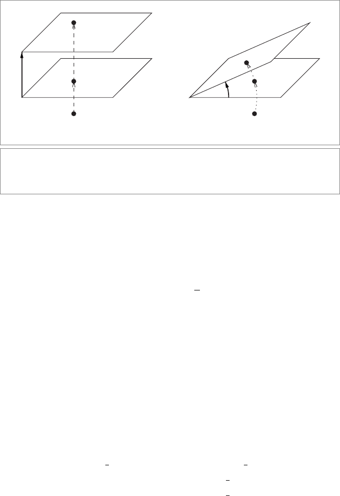
motions. We construct their versors, and illustrate this in Figure 13.1.

•

Translations. As a special case of versor composition, we compute the product of

two reﬂecting parallel planes with the same direction but at a differing location, as

in Figure 13.1(a). Let n be their unit normal vector, then we compute

(n + δ

∞)(n + δ

∞) = 1 − (δ

− δ

) n ∞≡1 − t∞/2 ≡ T

where we deﬁne the Euclidean translation vector t ≡ 2(δ

− δ

)n. Geometrically,

we would expect this double reﬂection to represent a translation in the direction n,

over twice the distance of the reﬂecting planes (i.e., over t).

For a point at the (arbitrary) origin o, this behavior is easily checked:

−1

= (1 − t ∞/2) o (1 + t ∞/2)

= o −

(t ∞ o − o t ∞) − t ∞ o t ∞/4

= o − t (∞·o) −∞(2o ·∞−∞o) t

= o + t +

∞≡t.

(Verify this computation carefully, as it contains techniques you will frequently use.)

This is the representative of the point t at location t relative to the origin o,sowe

366 THE CONFORMAL MODEL: OPERATIONAL EUCLIDEAN GEOMETRY CHAPTER 13

(a) (b)

φ/2

t/2

Figure 13.1: The versors for the Euclidean transformations can be constructed as multi-

ple reﬂections in well-chosen planes. (a) Two parallel planes make a translation, and (b) two

intersecting planes make a rotation.

have indeed found the translation versor. This versor is even a rotor, for T



(1 − t ∞/2) (1 + t ∞/2) = 1 − t ∞ t ∞/4 = 1 + t

∞

/4 = 1.

Like all rotors in

n+1,1

, the translation rotor has an exponential representation.

This is easy to construct from the fact that ∞ squares to 0:

= 1 − t ∞/2 = 1 + (−t∞/2) +

(−t∞/2)

+ ··· = e

−t∞/2

The Taylor expansion of the exponential truncates by itself, after the ﬁrst-order

term. We foresaw such unusual rotors when discussing the exponential in Sec-

tion 7.4.2.

•

Rotations in the Origin. If we consider two planes in the origin as in Figure 13.1(b),

these are dually represented as the purely Euclidean vectors π

= n

and π

. Viewed as reﬂection versors, we may take these as unit vectors without loss of

generality. Their product is the versor

= n

in which we recognize the purely Euclidean rotor R. Let us check what it does on a

point, represented as a vector of R

n+1,1

R (o + p +

∞)R

−1

= RoR

−1

+ R p R

−1

(R ∞ R

−1

)

= o + (R p R

−1

) +

∞

= o + (R p R

−1

) +

(R pR

−1

)

∞,

which holds simply because the elements o and ∞ commute with the purely

Euclidean elements. This is indeed the representation of the point at location

SECTION 13.2 EUCLIDEAN TRANSFORMATIONS AS VERSORS 367

R p R

−1

, so successive reﬂections in planes through the origin are a rotation in a

plane through the origin. This was also the case in the vector space model when we

introduced its rotors in Chapter 7 (and therefore also in the homogeneous model).

This rotor representation of rotations is therefore nicely backwards compatible: it is

literally the same as in the vector space model contained in the space

n+1,1

, and it

merely acts on the whole space now.

Since this rotor is completely Euclidean, the earlier results of Chapter 7 and the

vector space model in Chapter 10 apply, and we can write it as

R = e

−I␾/2

= cos(␾/2) − sin(␾/2) I

in terms of its rotation plane I and rotation angle ␾.

•

General Rigid Body Motions. A general rigid body motion can be constructed by

ﬁrst doing a rotation in the origin and following it by a translation. That gives a

rotor of the form

(1 − t∞/2) R.

This generally contains terms of grades 0, 2, and 4. Being a rotor, the general rigid

body motion can also be written in exponential form, but this is a bit involved: it

requires viewing it as a screw motion (i.e., a rotation around a general axis combined

with a translation along that axis). We will get back to analyzing and interpreting

such motions in Section 13.5.2.

The above shows how the Euclidean proper motions are represented as rotors (i.e., as even

unit versors). Improper Euclidean motions can be represented by odd unit versors (just

multiply by a vector representing a dual reﬂection plane).

As a shorthand of the linear transformation produced by the application of T

in a versor

product, we will use

[·] (note the sans serif font). For the linear transformation of the

rotor R

I␾

, we may use the notation R

I␾

[·] (though we may conveniently drop the reference

to the bivector angle).

13.2.3 COVARIANT PRESERVATION OF STRUCTURE

By representing Euclidean transformations as versors, we have achieved an important

algebraic milestone in computing with Euclidean spaces, with far-reaching geometric

consequences: automatic structure-preservation of all our constructions, in the sense of

Section 7.6.3. By this we mean that a construction made anywhere, in any orientation,

will automatically transform properly under a Euclidean motion.

As an example, we have just seen how we make a rotation by reﬂection in two planes

passing through a point o as the product R = π

. If we now would want to have a

similar rotation at a point p, we could deﬁne that new rotation by moving both planes to

p by a translation versor T

and making the computation π

for the moved planes

368 THE CONFORMAL MODEL: OPERATIONAL EUCLIDEAN GEOMETRY CHAPTER 13

≡ T

−1

and π

≡ T

−1

. But when we do this, we ﬁnd that this is the same as

applying the translation T

to the original rotor R, for π

= T

−1

= T

−1

. The rotor of the moved planes is the moved rotor of the planes!

This is of course what we want for our original construction to be geomet rically meaning-

ful: it should transfer to another location in precisely this covariant manner (co-variant,

implying: varying with the change) under the transformations of Euclidean geomet ry. We

have effectively used similarity under Euclidean transformations as a generative principle

rather than as a property to check afterwards.

It should be clear from this example that it is precisely the versor representation that makes

this covariant structure preservation work so automatically, and that it should therefore

work for any Euclidean transformation (since they are all represented by versors in the

conformal model). We discuss the abstract principle involved in some detail, so that we

can apply it throughout the remainder of this chapter. The most important structure-

preservation properties of the versor product are easily proved.

•

The versor product preserves the structure of a geometric product:

V[XY] = V[X] V[Y].

Proof:

Use associativity: V (XY) V

−1

= VXYV

−1

= VXV

−1

VYV

−1

(VXV

−1

)(VYV

−1

•

Theversorproductislinear:

V[α X + β Y] = α V[X] + β V[Y].

Proof: V (α X + β Y) V

−1

= α VXV

−1

+ β VYV

−1

•

Theversorproductisgrade-preserving:

V[X]

= V[X

Proof: Grades are deﬁned in terms of the number of factors in an outer product.

An outer product can be written as a sum of geometric products, and under trans-

formation each of its terms transforms in a structure-preserving manner. The fac-

torization of the transform is the transform of the factorization, and therefore the

number of (transformed) vector factors in the outer product is preserved.

In Part I, we saw that we construct all objects and operators in geometric algebra using

only these constructive elements (either as linear combinations of geometric products or

by grade selection). Therefore the versors preserve all constructions, even including

meet

and join, inverses, and duality. So the universal structure preservation of constructions

can be denoted compactly as

V (A ◦ B) V

−1

= (VAV

−1

) ◦ (VBV

−1

where ◦ may be substituted by any of the products ∧, , , ∗, ∩, ∪.

4 For structural clarity, we suppressed the signs in (7.18), which really should be there. You can easily verify that

the result still holds when these are included.

SECTION 13.2 EUCLIDEAN TRANSFORMATIONS AS VERSORS 369

This leads to the operational model principle, of which the conformal model is merely

one manifestation:

If we have managed to construct a geometric algebra in which useful transformations

(motions) in the base space are represented as versors, then all constructions in the

model transform covariantly (i.e., with preservation of their structure).

We implicitly used this principle for rotations in the vector space model, which is why that

is the operational model for directions in space. The homogeneous model aug mented it

with translations as linear transformations, but not as versors, which is why it had some

problems preserving the structure of constructions (notably the metric properties). In

the conformal model we ﬁnally have the Euclidean transformations as versors, so all con-

structions should be covariant under Euclidean transformations. It is the smallest known

model that can do this. Operational models for other important geometries (such as pro-

jective geometry) have yet to be developed.

13.2.4 THE INVARIANCE OF PROPERTIES

Structure preservation is useful in analyzing and constructing all elements in the conformal

model: it saves work. Since we have the Euclidean transformations available, we need to

focus only on standardized elements at the origin (which is arbitrary anyway) to determine

their form and deﬁning equations. We can always move them to their desired location and

orientation later. But are we guaranteed that their deﬁning properties are preserved under

such a transformation? For instance, could a point become a dual sphere or a dual plane?

They are all represented as vectors, and could these not change into each other?

This brings us to how the characteristic properties change, that determine the interpre-

tation of a representative element. For vectors, these proper ties were given in Table 13.2.

They express that some combination of products is equal to a scalar. That algebraic form

already guarantees that they are structurally preserved. To take an example, we have seen

above how a unit point t at location t can be made by translation of a unit point at the

origin: t = T

−1

. But how do we know that it is still a unit point and not a dual sphere

or dual plane? Of the original point o, we knew that o

= 0 and −∞ · o = 1. Since these

conditions are completely expressed in terms of the products of geometric algebra, they

transform covariantly under the Euclidean transformation of translation, so we can relate

the properties of t to those of o:

tt= T

−1

= T

ooT

−1

= T

0 T

−1

= 0,

so indeed, t is also a point. Moreover,

−∞ · t = −∞ · (T

−1

) = −(T

∞ T

−1

) · (T

−1

) = −T

(∞·o) T

−1

= 1,

so t also has unit weight. Note that in the der ivation of weight preservation, it is essential

that ∞ is an invariant of the translation: it does not change, so the normalization equation

preserves its form after transformation.

370 THE CONFORMAL MODEL: OPERATIONAL EUCLIDEAN GEOMETRY CHAPTER 13

Characteristic properties expressed as scalar conditions in terms of the products and ∞

are automatically invariants of the Euclidean transformations.

In summary, as long as we construct elements and their deﬁning properties in terms

of the products of the geometric algebra of the operational model

n+1,1

,weare

automatically guaranteed of their covariance (for the elements) and invariance (for

their properties) under Euclidean transformations. So we can construct everything

around the origin, and yet get a full inventory of the general possibilities. With that

labor-saving capability, we are ready to construct and inter pret general blades of

n+1,1

effectively.

13.3 FLATS AND DIRECTIONS

Let us embed the geometrical elements of the homogeneous model into the conformal

model, and investigate how the versor properties empower our geometr ic representation.

We originally started our exploration of the conformal model in Section 13.1.3 by

interpreting vectors, which turned out to be the dual representations of spheres (real,

imaginary, or zero radius), hyperplanes, and the point at inﬁnity. To establish the

correspondence with the vector space model and the homogeneous model, we now

prefer instead to construct the direct representations of elements. The two repre-

sentations are of course related by duality, so none is more fundamental than the

other, but it is more natural to assign orientations to ﬂats (and spheres) in the direct

representation—and then dualization automatically introduces some grade-dependent

orientation signs in their corresponding duals, which are good to get straight once and

for all.

Constructing direct representations implies that we use the outer product ∧, both for con-

structing the elements (as blades A) and for testing what Euclidean point set it represents

(by solving x ∧ A = 0).

13.3.1 THE DIRECT REPRESENTATION OF FLATS

We start constructing an element of the form

X = α (p

∧ p

∧···∧p

∧∞),

by which we mean the weighted outer product of k+1 unit points and the point at inﬁnity

∞. This clearly contains the point at inﬁnity (since ∞∧X = 0), and we will ﬁnd out that

such a blade is the direct representation of a k-ﬂat in the conformal model (i.e., an offset

k-dimensional linear subspace of

). We do so by rewriting the blade to a form that we

mostly recognize from the homogeneous model. This is done in three steps: standardiza-

tion, interpretation, and generalization.

SECTION 13.3 FLATS AND DIRECTIONS 371

Standardization

By the structure preservation principle, we still have the general form if we take p

to be

the arbitrary origin o (and we can view this either as moving the whole blade X back to

the origin to make p

coincide with o, or as choosing p

as the origin of our representa-

tion). Note that the invariance of ∞ is essential (if it changed under translation, the form

of the expression would not be the same at the origin). So we have reduced the element

X to

X = α (o ∧ p

∧···∧p

∧∞).

Now because the outer product is antisymmetric, we can subtract one of the factors from

each of the others without changing the value of the product (the extra terms would pro-

duce zero, a∧b = a ∧ (b−a) being the prime example). We subtract o, and get the element

X into the form:

X = α



o ∧ (p

− o) ∧···∧(p

− o) ∧∞



We substitute the general form of the point representation of (13.3), setting p

= o + p

∞, to obtain:

X = α



o ∧ (p

∞) ∧···∧(p

∞) ∧∞



The outer product with ∞ eliminates the extra terms

∞.Sowehave:

X = α (o ∧ p

∧···∧p

∧∞).

We can now reduce the part involving the vectors p

to a purely Euclidean k-blade A

, into

which we also absorb the weight α, deﬁning A

= α p

∧···∧p

. We therefore ultimately

ﬁnd that this class of blade is equivalent to:

X = o ∧ A

∧∞,

a much simpliﬁed form.

Interpretation

To ﬁnd the Euclidean interpretation of X = o ∧ A

∧∞as a direct blade, we probe it with

a point x and solve x ∧ (o ∧ A

∧∞) = 0; that should give the set of Euclidean points it

represents. Let us bring this into a more familiar form by expanding x as o + x +

∞.

We immediately realize that the outer products with o and ∞ eliminate the ﬁrst and last

term of this point representation, so we effectively can substitute x = x without changing

the solution:

0 = x ∧ o ∧ A

∧∞= x ∧ o ∧ A

∧∞.

Therefore we need to solve x ∧ o ∧ A

∧∞ = 0. This equation contains a purely Euclidean

part (x ∧ A

) and a non-Euclidean part (o ∧∞). These are orthogonal, so that their outer