Engelbrecht Andries P. Computational Intelligence: An Introduction

Подождите немного. Документ загружается.

58 4. Unsupervised Learning Neural Networks



p=1

k,p

/P (4.8)

Another variant of the Hebbian learning rule uses the correlation in the changes in

activation values over consecutive time steps. For this learning rule, referred to as

differential Hebbian learning,

∆u

(t)=η∆z

(t)∆o

(t − 1) (4.9)

where

∆z

(t)=z

i,p

(t) − z

i,p

(t − 1) (4.10)

and

∆o

(t − 1) = o

k,p

(t − 1) − o

k,p

(t − 2) (4.11)

4.3 Principal Component Learning Rule

Principal component analysis (PCA) [426] is a statistical technique used to transform

a data space into a smaller space of the most relevant features. The aim is to project

the original I-dimensional space onto an I



-dimensional linear subspace, where I



I, such that the variance in the data is maximally explained within the smaller I



dimensional space. Features (or inputs) that have little variance are thereby removed.

The principal components of a data set are found by calculating the covariance (or

correlation) matrix of the data patterns, and by getting the minimal set of orthogonal

vectors (the eigenvectors) that span the space of the covariance matrix. Given the

set of orthogonal vectors, any vector in the space can be constructed with a linear

combination of the eigenvectors.

Oja developed the ﬁrst principal components learning rule, with the aim of extract-

ing the principal components from the input data [635]. Oja’s principal components

learning rule is an extension of the Hebbian learning rule, referred to as normalized

Hebbian learning, to include a feedback term to constrain weights. In doing so, prin-

cipal components could be extracted from the data. The weight change is given as

∆u

(t)=u

i(t) − u

(t − 1)

= ηo

k,p

i,p

− o

k,p

(t − 1)]

= ηo

k,p

i,p

  

Hebbian

− ηo

k,p

(t − 1)



 

forgetting factor

(4.12)

The ﬁrst term corresponds to standard Hebbian learning (refer to equation (4.2)),

while the second term is a forgetting factor to prevent weight values from becoming

unbounded.

The value of the learning rate, η, above is important to ensure convergence to a stable

state. If η is too large, the algorithm will not converge due to numerical unstability.

If η is too small, convergence is extremely slow. Usually, the learning rate is time

4.4 Learning Vector Quantizer-I 59

dependent, starting with a large value that decays gradually as training progresses.

To ensure numerical stability of the algorithm, the learning rate η

(t) for output unit

must satisfy the inequality:

0 <η

(t) <

1.2λ

(4.13)

where λ

is the largest eigenvalue of the covariance matrix of the inputs to the unit

[636]. A good initial value is given as η

(0) = 1/[2Z

Z], where Z is the input matrix.

Cichocki and Unbehauen [130] provided an adaptive learning rate that utilizes a for-

getting factor, γ, as follows:

(t)=

(t−1)

+ o

(t)

(4.14)

with

(0) =

(0)

(4.15)

Usually, 0.9 ≤ γ ≤ 1.

The above can be adapted to allow the same learning rate for all the weights in the

following way:

(t)=

(t−1)

+ ||o(t)||

(4.16)

with

(0) =

||o(0)||

(4.17)

Sanger [756] developed another principal components learning algorithm, similar to

that of Oja, referred to as generalized Hebbian learning. The only diﬀerence is the

inclusion of more feedback information and a decaying learning rate η(t):

∆u

(t)=η(t)[z

i,p

k,p

  

Hebbian

−o

k,p



j=0

(t − 1)o

j,p

] (4.18)

For more information on principal component learning, the reader is referred to the

summary in [356].

4.4 Learning Vector Quantizer-I

One of the most frequently used unsupervised clustering algorithms is the learning

vector quantizer (LVQ) developed by Kohonen [472, 474]. While several versions of

LVQ exist, this section considers the unsupervised version, LVQ-I.

Ripley [731] deﬁned clustering algorithms as those algorithms where the purpose is to

divide a set on n observations into m groups such that members of the same group

60 4. Unsupervised Learning Neural Networks

are more alike than members of diﬀerent groups. The aim of a clustering algorithm is

therefore to construct clusters of similar input vectors (patterns), where similarity is

usually measured in terms of Euclidean distance. LVQ-I performs such clustering.

The training process of LVQ-I to construct clusters is based on competition. Referring

to Figure 4.1, each output unit o

represents a single cluster. The competition is among

the cluster output units. During training, the cluster unit whose weight vector is the

“closest” to the current input pattern is declared as the winner. The corresponding

weight vector and that of neighboring units are then adjusted to better resemble the

input pattern. The “closeness” of an input pattern to a weight vector is usually

measured using the Euclidean distance. The weight update is given as

∆u

(t)=



η(t)[z

i,p

− u

(t − 1)] if k ∈ κ

k,p

(t)

0otherwise

(4.19)

where η(t) is a decaying learning rate, and κ

k,p

(t) is the set of neighbors of the winning

cluster unit o

for pattern p. It is, of course, not strictly necessary that LVQ-I makes

use of a neighborhood function, thereby updating only the weights of the winning

output unit.

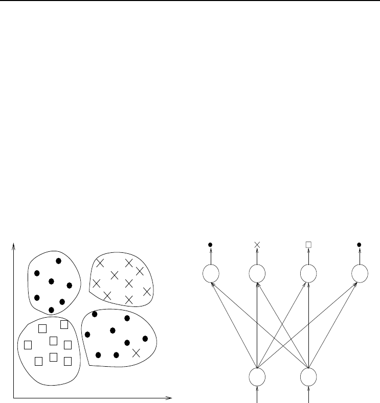
(a) Clustering Problem

1234

(b) LVQ-I network

Figure 4.2 Learning Vector Quantizer to Illustrate Clustering

An illustration of clustering, as done by LVQ-I, is given in Figure 4.2. The input

space, deﬁned by two input units z

and z

, is represented in Figure 4.2(a), while

Figure 4.2(b) illustrates the LVQ-I network architecture required to form the clusters.

Note that although only three classes exist, four output units are necessary – one for

each cluster. Less output units will lead to errors since patterns of diﬀerent classes

will be grouped in the same cluster, while too many clusters may cause overﬁtting.

For the problem illustrated in Figure 4.2(a), an additional cluster unit may cause a

separate cluster to learn the single × in cluster 4.

The Kohonen LVQ-I algorithm is summarized in Algorithm 4.2. For the LVQ-I, weights

are either initialized to random values, sampled from a uniform distribution, or by

4.4 Learning Vector Quantizer-I 61

Algorithm 4.2 Learning Vector Quantizer-I Training Algorithm

Initialize the network weights, the learning rate, and the neighborhood radius;

while stopping condition(s) not true do

for each pattern p do

Compute the Euclidean distance, d

k,p

, between input vector z

and each

weight vector u

=(u

, ···,u

)as

k,p

, u









i=1

i,p

−u

)

(4.20)

Find the output unit o

for which the distance d

k,p

is the smallest;

Update all the weights for the neighborhood κ

k,p

using equation (4.19);

end

Update the learning rate;

Reduce the neighborhood radius at speciﬁed learning iterations;

end

taking the ﬁrst input patterns as the initial weight vectors. For the example in Fig-

ure 4.2(b), the latter will result in the weights u

= z

1,1

= z

2,1

= z

1,2

2,2

,etc.

Stopping conditions may be

• a maximum number of epochs is reached,

• stop when weight adjustments are suﬃciently small,

• a small enough quantization error has been reached, where the quantization error

is deﬁned as



p=1

||z

− u

(4.21)

One problem that may occur in LVQ networks is that one cluster unit may dominate

as the winning cluster unit. The danger of such a scenario is that most patterns will

be in one cluster. To prevent one output unit from dominating, a “conscience” factor

is incorporated in a function to determine the winning output unit. The conscience

factor penalizes an output for winning too many times. The activation value of output

units is calculated using

k,p



1formin

∀k

k,p

, u

) − b

(t)}

0otherwise

(4.22)

where

(t)=γ(

− g

(t)) (4.23)

and

(t)=g

(t − 1) + β(o

k,p

− g

(t − 1)) (4.24)

62 4. Unsupervised Learning Neural Networks

In the above, d

k,p

is the Euclidean distance as deﬁned in equation (4.20), I is the total

number of input units, and g

(0) = 0. Thus, b

(0) =

, which initially gives each

output unit an equal chance to be the winner; b

(t) is the conscience factor deﬁned

for each output unit. The more an output unit wins, the larger the value of g

(t)

becomes, and b

(t) becomes larger negative. Consequently, a factor |b

(t)| is added to

the distance d

k,p

. Usually, for normalized inputs, β =0.0001 and γ = 10.

4.5 Self-Organizing Feature Maps

Kohonen developed the self-organizing feature map (SOM) [474, 475, 476], as moti-

vated by the self-organization characteristics of the human cerebral cortex. Studies of

the cerebral cortex showed that the motor cortex, somatosensory cortex, visual cortex

and auditory cortex are represented by topologically ordered maps. These topological

maps form to represent the structures sensed in the sensory input signals.

The self-organizing feature map is a multidimensional scaling method to project an

I-dimensional input space to a discrete output space, eﬀectively performing a com-

pression of input space onto a set of codebook vectors. The output space is usually a

two-dimensional grid. The SOM uses the grid to approximate the probability density

function of the input space, while still maintaining the topological structure of input

space. That is, if two vectors are close to one another in input space, so is the case

for the map representation.

The SOM closely resembles the learning vector quantizer discussed in the previous

section. The diﬀerence between the two unsupervised algorithms is that neurons are

usually organized on a rectangular grid for SOM, and neighbors are updated to also

perform an ordering of the neurons. In the process, SOMs eﬀectively cluster the

input vectors through a competitive learning process, while maintaining the topological

structure of the input space.

Section 4.5.1 explains the standard stochastic SOM training rule, while a batch version

is discussed in Section 4.5.2. A growing approach to SOM is given in Section 4.5.3.

Diﬀerent approaches to speed up the training of SOMs are overviewed in Section 4.5.4.

Section 4.5.5 explains the formation of clusters for visualization purposes. Section 4.5.6

discusses in brief diﬀerent ways how the SOM can be used after training.

4.5.1 Stochastic Training Rule

SOM training is based on a competitive learning strategy. Assume I-dimensional

input vectors z

, where the subscript p denotes a single training pattern. The ﬁrst

step of the training process is to deﬁne a map structure, usually a two-dimensional

grid (refer to Figure 4.3). The map is usually square, but can be of any rectangular

shape. The number of elements (neurons) in the map is less than the number of

training patterns. Ideally, the number of neurons should be equal to the number of

independent training patterns.

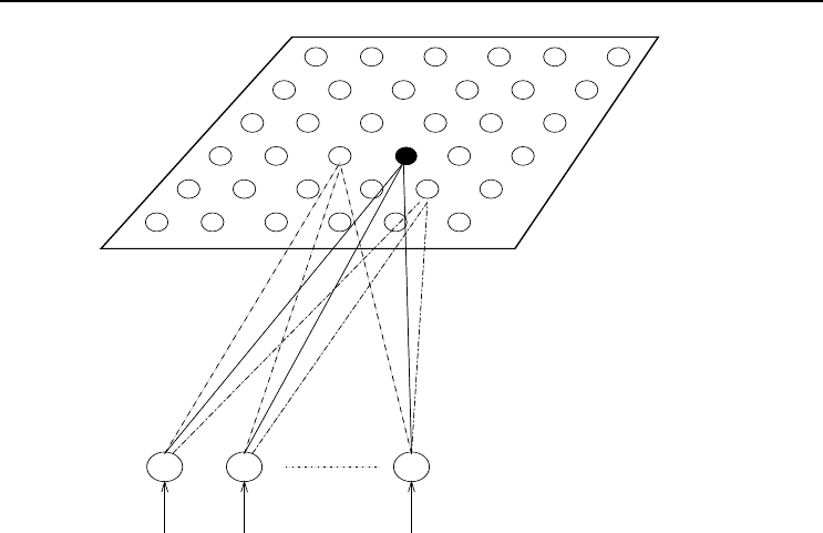
4.5 Self-Organizing Feature Maps 63

Map

Input Vector

Figure 4.3 Self-organizing Map

Each neuron on the map is associated with and I-dimensional weight vector that forms

the centroid of one cluster. Larger cluster groupings are formed by grouping together

“similar” neighboring neurons.

Initialization of the codebook vectors can occur in various ways:

• Assign random values to each weight w

=(w

kj1

kj2

, ···,w

KJI

), with K the

number of rows and J the number of columns of the map. The initial values

are bounded by the range of the corresponding input parameter. While random

initialization of weight vectors is simple to implement, this form of initialization

introduces large variance components into the map which increases training time.

• Assign to the codebook vectors randomly selected input patterns. That is,

= z

(4.25)

with p ∼ U(1,P

This approach may lead to premature convergence, unless weights are perturbed

with small random values.

• Find the principal components of the input space, and initialize the codebook

vectors to reﬂect these principal components.

• A diﬀerent technique of weight initialization is due to Su et al. [818], where

the objective is to deﬁne a large enough hyper cube to cover all the training

patterns [818]. The algorithm starts by ﬁnding the four extreme points of the

map by determining the four extreme training patterns. Firstly, two patterns

are found with the largest inter-pattern Euclidean distance. A third pattern is

64 4. Unsupervised Learning Neural Networks

located at the furthest point from these two patterns, and the fourth pattern

with largest Euclidean distance from these three patterns. These four patterns

form the corners of the map. Weight values of the remaining neurons are found

through interpolation of the four selected patterns, in the following way:

– Weights of boundary neurons are initialized as

− w

J −1

(j − 1) + w

(4.26)

− w

J −1

(j − 1) + w

(4.27)

−w

K −1

(k − 1) + w

(4.28)

− w

K −1

(k − 1) + w

(4.29)

for all j =2, ···,J − 1andk =2, ···,K− 1.

– The remaining codebook vectors are initialized as

− w

J −1

(j − 1) + w

(4.30)

for all j =2, ···,J − 1andk =2, ···,K− 1.

The standard training algorithm for SOMs is stochastic, where codebook vectors are

updated after each pattern is presented to the network. For each neuron, the associated

codebook vector is updated as

(t +1)=w

(t)+h

mn,kj

(t)[z

− w

(t)] (4.31)

where mn is the row and column index of the winning neuron. The winning neuron is

found by computing the Euclidean distance from each codebook vector to the input

vector, and selecting the neuron closest to the input vector. That is,

||w

− z

=min

∀kj

{||w

− z

} (4.32)

The function h

mn,kj

(t) in equation (4.31) is referred to as the neighborhood function.

Thus, only those neurons within the neighborhood of the winning neuron mn have

their codebook vectors updated. For convergence, it is necessary that h

mn,kj

(t) → 0

when t →∞.

The neighborhood function is usually a function of the distance between the coordi-

nates of the neurons as represented on the map, i.e.

mn,kj

(t)=h(||c

− c

,t) (4.33)

with the coordinates c

∈ R

. With increasing value of ||c

− c

(that is,

neuron kj is further away from the winning neuron mn), h

mn,kj

→ 0. The neighbor-

hood can be deﬁned as a square or hexagon. However, the smooth Gaussian kernel is

mostly used:

mn,kj

(t)=η(t)e

−

||c

−c

2σ

(t)

(4.34)

4.5 Self-Organizing Feature Maps 65

where η(t) is the learning rate and σ(t) is the width of the kernel. Both η(t)andσ(t)

are monotonically decreasing functions.

The learning process is iterative, continuing until a “good” enough map has been

found. The quantization error is usually used as an indication of map accuracy, deﬁned

as the sum of Euclidean distances of all patterns to the codebook vector of the winning

neuron, i.e.



p=1

||z

− w

(t)||

(4.35)

Training stops when E

is suﬃciently small.

4.5.2 Batch Map

The stochastic SOM training algorithm is slow due to the updates of weights after each

pattern presentation: all the weights are updated. Batch versions of the SOM training

rule have been developed that update weight values only after all patterns have been

presented. The ﬁrst batch SOM training algorithm was developed by Kohonen [475],

and is summarized in Algorithm 4.3.

Algorithm 4.3 Batch Self-Organizing Map

Initialize the codebook vectors by assigning the ﬁrst KJ training patterns to them,

where KJ is the total number of neurons in the map;

while stopping condition(s) not true do

for each neuron, kj do

Collect a list of copies of all patterns z

whose nearest codebook vector

belongs to the topological neighborhood of that neuron;

end

for each codebook vector do

Compute the codebook vector as the mean over the corresponding list of

patterns;

end

Based on the batch learning approach above, Kaski et al. [442] developed a faster

version, as summarized in Algorithm 4.4.

4.5.3 Growing SOM

One of the design problems when using a SOM is deciding on the size of the map. Too

many neurons may cause overﬁtting of the training patterns, with each training pattern

assigned to a diﬀerent neuron. Alternatively, the ﬁnal SOM may have succeeded in

forming good clusters of similar patterns, but with many neurons with a zero or close

to zero frequency. The frequency of a neuron refers to the number of patterns for

66 4. Unsupervised Learning Neural Networks

Algorithm 4.4 Fast Batch Self-Organizing Map

Initialize the codebook vectors, w

, using any initialization approach;

while stopping condition(s) not true do

for each neuron, kj do

Compute the mean over all patterns for which that neuron is the winner;

Denote the average by

;

end

Adapt the weight values for each codebook vector using



nm,kj



nm,kj

(4.36)

where nm iterates over all neurons, N

is the number of patterns for which

neuron nm is the winner, and h

nm,kj

is the neighborhood function which

indicates if neuron nm is in the neighborhood of neuron kj, and to what degree.

end

which that neuron is the winner, referred to as the best matching neuron (BMN). Too

many neurons also cause a substantial increase in computational complexity. Too few

neurons, on the other hand, will result in clusters with a high variance among the

cluster members.

An approach to ﬁnd near optimal SOM architectures is to start training with a small

architecture, and to grow the map when more neurons are needed. One such SOM

growing algorithm is given in Algorithm 4.5, assuming a square map structure. Note

that the map-growing process coexists with the training process.

Growing of the map is stopped when any one of the following criteria is satisﬁed:

• the maximum map size has been reached;

• the largest neuron quantization error is less than a user speciﬁed threshold, ;

• the map has converged to the speciﬁed quantization error.

A few aspects of the growing algorithm above need some explanation. These are the

constants , γ, and the maximum map size as well as the diﬀerent stopping conditions.

A good choice for γ is 0.5. The idea of the interpolation step is to assign a weight

vector to the new neuron ab such that it removes patterns from neuron kj with the

largest quantization erro in order to reduce the error of that neuron. A value less than

0.5 will position neuron ab closer to kj, with the chance that more patterns will be

removed from neuron kj. A value larger than 0.5 will have the opposite eﬀect.

The quantization error threshold, , is important to ensure that a suﬃcient map size

is constructed. A small value for  may result in a too large map architecture, while

a too large  may result in longer training times to reach a large enough architecture.

An upper bound on the size of the map is easy to determine: it is simply the number

of training patterns, P

. This is, however, undesirable. The maximum map size is

4.5 Self-Organizing Feature Maps 67

Algorithm 4.5 Growing Self-Organizing Map Algorithm

Initialize the codebook vectors for a small, undersized SOM;

while stopping condition(s) not true do

while growing condition not triggered do

Train the SOM for t



pattern presentations using any SOM training method;

end

if grow condition is met then

Find the neuron kj with the largest quantization error;

Find the furthest immediate neighbor mn in the row-dimension of the map,

and the furthest neuron rs in the column-dimension;

Insert a column between neurons kj and rs and a row between neurons kj

and mn (this step preserves the square structure of the map);

For each neuron ab in the new column, initialize the corresponding codebook

vectors w

using

= γ(w

a,b−1

+ w

a,b+1

) (4.37)

and for each neuron in the new row,

= γ(w

a−1,b

+ w

a+1,b

) (4.38)

where γ ∈ (0, 1)

end

Reﬁne the weights of the ﬁnal SOM architecture with additional training steps until

convergence has been reached.

rather expressed as βP

,withβ ∈ (0, 1). Ultimately, the map size should be at least

equal to the number of independent variables in the training set. The optimal value

of β is problem dependent, and care should be taken to ensure that β is not too small

if a growing SOM is not used. If this is the case, the ﬁnal map may not converge to

the required quantization error since the map size will be too small.

4.5.4 Improving Convergence Speed

Training of SOMs is slow, due to the large number of weight updates involved (all

the weights are updated for standard SOM training). Several mechanisms have been

developed to reduce the number of training calculations, thereby improving speed

of convergence. BatchMap is one such mechanism. Other approaches include the

following:

Optimizing the neighborhood

If the Gaussian neighborhood function as given in equation (4.34) is used, all neurons

will be in the neighborhood of the BMN, but to diﬀerent degrees, due to the asymptotic