Engelbrecht Andries P. Computational Intelligence: An Introduction

Подождите немного. Документ загружается.

78 5. Radial Basis Function Networks

Algorithm 5.2 Gradient Descent Training of RBFNN

Select the number of centers, J;

for j =1,...,J do

p ∼ U(1,P

);

(t)=z

;

(t)=

max

√

;

end

for k =1,...,K do

for j =1,...,J do

∼ U(w

min

max

);

end

while stopping condition(s) not true do

Select an input pattern, d

=(z

, t

);

for k =1,...,K do

Compute o

k,p

using equation (5.3);

for j =1,...,J do

Compute weight adjustment step size,

∆w

(t)=−η

∂E

∂w

(t) (5.14)

Adjust weights using

(t +1)=w

(t)+∆w

(t) (5.15)

end

for j =1,...,J do

for i =1,...,I do

Compute center step size,

∆µ

(t)=−η

∂E

∂µ

(t) (5.16)

Adjust centers using

(t +1)=µ

(t)+∆µ

(t) (5.17)

end

Compute width step size,

∆σ

(t)=−η

∂E

∂σ

(t) (5.18)

Adjust widths using

(t +1)=σ

(t)+∆σ

(t) (5.19)

end

5.2 Radial Basis Function Neural Networks 79

Algorithm 5.3 Two-Phase RBFNN Training

Initialize w

,k=1,...,K and j =1,...,J;

Initialize µ

,j=1,...,J and i =1,...,I;

Initialize σ

,j=1,...,J;

while LVQ-I has not converged do

Apply one epoch of LVQ-I to adjust µ

,j=1,...,J;

Adjust σ

,j=1,...,J;

end

t =0;

while gradient descent has not converged do

Select an input pattern, (z

, t

);

Compute the weight step sizes,

∆w

(t)=η



k=1

k,p

− o

k,p

j,p

(5.20)

Adjust the weights,

(t +1)=w

(t)+∆w

(t) (5.21)

end

Before the LVQ-I training phase, the RBFNN is initialized as follows:

• The centers are initialized by setting all the µ

weights to the average value of

all inputs in the training set.

• The weights are initialized by setting all σ

to the standard deviation of all input

values over the training set.

• The hidden-to-output weights, w

, are initialized to small random values.

At the end of each LVQ-I iteration, basis function widths are recalculated as follows:

For each hidden unit, ﬁnd the average of the Euclidean distances between µ

and the

input patterns for which the hidden unit was selected as the winner. The width, σ

is set to this average.

Instead of using LVQ-I, Moody and Darken [605] uses K-means clustering in the ﬁrst

phase. The K-means algorithm is initialized by setting each µ

to a randomly selected

input pattern. Training patterns are assigned to their closest center, after which each

center is recomputed as



p∈C

(5.22)

where C

is the set of patterns closest to center µ

. Training patterns are again

reassigned to their closest center, after which the centers are recalculated. This process

continues until there is no signiﬁcant change in the centers.

80 5. Radial Basis Function Networks

After the K-means clustering, the widths are determined as follow:

= τ||µ

− µ

|| (5.23)

where µ

is the nearest neighbor of µ

,andτ ∈ [1, 1.5].

The second-phase is then executed to learn the weight values, w

using gradient

descent, or by solving for w

as in equation (5.12).

5.2.4 Radial Basis Function Network Variations

Two variations of the standard RBFNN are discussed in this section. These variations

were developed as an attempt to improve the performance of RBFNNs.

Normalized Hidden Unit Activations

Moody and Darken [605] proposed that hidden unit activations must be normalized

using,

j,p

Φ(||z

− µ

,σ

)



l=1

Φ(||z

− µ

,σ

)

(5.24)

This introduces the property that



j=1

j,p

)=1, ∀p =1,...,P

(5.25)

which means that the above normalization represents the conditional probability of

hidden unit j generating z

. This probability is given as

P (j|z

)



l=1

)

j,p

)



l=1

l,p

)

(5.26)

Soft-Competition

The K-means clustering approach proposed by Moody and Darken can be considered

as a hard competition winner-takes-all action. An input pattern is assigned to the

cluster of patterns of the µ

to which the input pattern is closest. Adjustment of µ

is then based only on those patterns for which it was selected as the winner.

In soft-competition [632], all input vectors have an inﬂuence on the adjustment of all

centers. For each hidden unit,



p=1

P (j|z



p=1

P (j|z

)

(5.27)

where P (j|z

) is deﬁned in equation (5.26).

5.3 Assignments 81

5.3 Assignments

1. Compare the performance of an RBFNN and a FFNN on a

classiﬁcation problem from the UCI machine learning repository

(http://www.ics.uci.edu/~mlearn/MLRepository.html).

2. Compare the performance of the Gaussian and logistic basis functions.

3. Suggest an alternative to compute the hidden-to-output weights instead of using

GD.

4. Suggest an alternative to compute the input-to-hidden weights instead of using

LVQ-I.

5. Investigate alternative methods to initialize an RBF NN.

6. Is it crucial that all w

be initialized to small random values? Motivate your

answer.

7. Develop a PSO, DE, and EP algorithm to train an RBFNN.

Chapter 6

Reinforcement Learning

The last learning paradigm to be discussed is that of reinforcement learning (RL) [823],

with its origins in the psychology of animal learning. The basic idea is that of awarding

the learner (agent) for correct actions, and punishing wrong actions. Intuitively, RL is

a process of trial and error, combined with learning. The agent decides on actions based

on the current environmental state, and through feedback in terms of the desirability

of the action, learns which action is best associated with which state. The agent learns

from interaction with the environment.

While RL is a general learning paradigm in AI, this chapter focuses on the role that

NNs play in RL. The LVQ-II serves as one example where RL is used to train a NN

to perform data clustering (refer to Section 5.1).

Section 6.1 provides an overview of RL. Model-free learning methods are given in

Section 6.2. Connectionist approaches to RL are described in Section 6.3.

6.1 Learning through Awards

Formally deﬁned, reinforcement learning is the learning of a mapping from situations

to actions with the main objective to maximize the scalar reward or reinforcement

signal [824]. Informally, reinforcement learning is deﬁned as learning by trial-and-

error from performance feedback from the environment or an external evaluator. The

agent has absolutely no prior knowledge of what action to take, and has to discover

(or explore) which actions yield the highest reward.

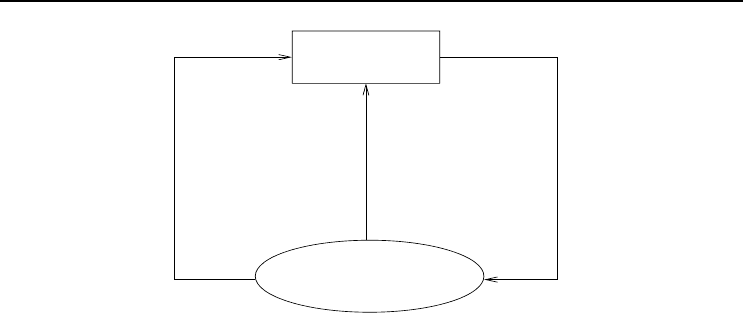
A typical reinforcement learning problem is illustrated in Figure 6.1. The agent re-

ceives sensory inputs from its environment, as a description of the current state of

the perceived environment. An action is executed, upon which the agent receives the

reinforcement signal or reward. This reward can be a positive or negative signal, de-

pending on the correctness of the action. A negative reward has the eﬀect of punishing

the agent for a bad action.

The action may cause a change in the agent’s environment, thereby aﬀecting the future

options and actions of the agent. The eﬀects of actions on the environment and future

states can not always be predicted. It is therefore necessary that the agent frequently

Computational Intelligence: An Introduction, Second Edition A.P. Engelbrecht

2007 John Wiley & Sons, Ltd

84 6. Reinforcement Learning

Learner

Environment

Reward

Action

Sensory

Input

Figure 6.1 Reinforcement Learning Problem

monitors its environment.

One of the important issues in RL (which occurs in most search methods) is that of

the exploration–exploitation trade-oﬀ. As already indicated, RL has two important

components:

• A trial and error search to ﬁnd good actions, which forms the exploration com-

ponent of RL.

• A memory of which actions worked well in which situations. This is the exploita-

tion component of RL.

It is important that the agent exploits what it has already learned, such that a reward

can be obtained. However, via the trial and error search, the agent must also explore

to improve action selections in the future.

A reinforcement learning agent has the following components:

• A policy, which is the decision making function of the agent. This function is

used to specify which action to execute in each of the situations that the agent

may encounter. The policy is basically a set of associations between actions and

situations, or alternatively, a set of stimulus-response rules.

• A reward function, which deﬁnes the goal of the agent. The reward function

deﬁnes what are good and bad actions for the agent for speciﬁc situations. The

reward is immediate, and represents only the current environment state. The

goal of the agent is to maximize the total reward that it receives over the long

run.

• A value function, which speciﬁes the goal in the long run. The value function

is used to predict future reward, and is used to indicate what is good in the long

run.

• Optionally, an RL agent may also have a model of the environment. The envi-

ronmental model mimics the behavior of the environment. This can be done by

transition functions that describe transitions between diﬀerent states.

6.1 Learning through Awards 85

For the value function, an important aspect is how the future should be taken into

account. A number of models have been proposed [432]:

• The finite-horizon model, in which the agent optimizes its expected reward

for the next n

steps, i.e.





t=1

r(t)



(6.1)

where r(t) is the reward for time-step t.

• The infinite-horizon discounted model, which takes the entire long-run

reward of the agent into consideration. However, each reward received in future

is geometrically discounted according to a discount factor, γ ∈ [0, 1):



∞



t=0

r(t)



(6.2)

The discount factor enforces a bound on the inﬁnite sum.

• The average reward model, which prefers actions that optimize the agent’s

long-run average reward:

lim

→∞





t=0

r(t)



(6.3)

A problem with this model is that it is not possible to distinguish between a

policy that gains a large amount of reward in the initial phases, and a policy

where the largest gain is obtained in the later phases.

In order to ﬁnd an optimal policy, π

∗

, it is necessary to ﬁnd an optimal value function.

A candidate optimal value function is [432],

∗

(s)=max

a∈A







R(s, a)+γ



∈S

T (s, a, s



∗



)







,s∈S (6.4)

where A is the set of all possible actions, S is the set of environmental states, R(s, a)

is the reward function, and T(s, a, s



) is the transition function. Equation (6.4) states

that the value of a state, s, is the expected instantaneous reward, R(s, a), for action

a plus the expected discounted value of the next state, using the best possible action.

From the above, a clear deﬁnition of the model in terms of the transition function,

T , and the reward function, R, is required. A number of algorithms have been de-

veloped for such RL problems. The reader is referred to [432, 824] for a summary of

these methods. Of more interest to this chapter are model-free learning methods, as

described in the next section.

86 6. Reinforcement Learning

6.2 Model-Free Reinforcement Learning Model

This section considers model-free RL methods, where the objective is to obtain an

optimal policy without a model of the environment. This section reviews two ap-

proaches, namely temporal diﬀerence (TD) learning (in Section 6.2.1) and Q-learning

(in Section 6.2.2).

6.2.1 Temporal Diﬀerence Learning

Temporal diﬀerence (TD) learning [824] learns the value policy using the update rule,

V (s)=V (s)+η(r + γV (s



) − V (s)) (6.5)

where η is a learning rate, r is the immediate reward, γ is the discount factor, s is the

current state, and s



is a future state. Based on equation (6.5), whenever a state, s,

is visited, its estimated value is updated to be closer to r + ηV (s



The above model is referred to as TD(0), where only one future step is considered.

The TD method has been generalized to TD(λ) strategies [825], where λ ∈ [0, 1] is a

weighting on the relevance of recent temporal diﬀerences of previous predictions. For

TD(λ), the value function is learned using

V (u)=V (u)+η(r + γV (s



) − V (s))e(u) (6.6)

where e(u) is the eligibility of state u. The eligibility of a state is the degree to which

the state has been visited in the recent past, computed as

e(s)=



(λγ)

t−t



s,s

(6.7)

where

s,s



1 s = s

0otherwise

(6.8)

The update in equation (6.6) is applied to every state, according to its eligibility, and

not just the previous state as for TD(0).

6.2.2 Q-Learning

In Q-learning [891], the task is to learn the expected discounted reinforcement values,

Q(s, a), of taking action a in state s, then continuing by always choosing actions

optimally. To relate Q-values to the value function, note that

∗

(s)=max

∗

(s, a) (6.9)

where V

∗

(s)isthevalueofs assuming that the best action is taken initially.

6.3 Neural Networks and Reinforcement Learning 87

The Q-learning rule is given as

Q(s, a)=Q(s, a)+η(r + γ max



∈A

Q(s



) − Q(s, a)) (6.10)

The agent then takes the action with the highest Q-value.

6.3 Neural Networks and Reinforcement Learning

Neural networks and reinforcement learning have been combined in a number of ways.

One approach of combining these models is to use a NN as an approximator of the

value function used to predict future reward [162, 432]. Another approach uses RL to

adjust weights. Both these approaches are discussed in this section.

As already indicated, the LVQ-II (refer to Section 5.1) implements a form of RL.

Weights of the winning output unit are positively updated only if that output unit

provided the correct response for the corresponding input pattern. If not, weights are

penalized through adjustment away from that input pattern. Other approaches to

use RL for NN training include RPROP (refer to Section 6.3.1), and gradient descent

on the expected reward (refer to Section 6.3.2). Connectionist Q-learning is used to

approximate the value function (refer to Section 6.3.3).

6.3.1 RPROP

Resilient propagation (RPROP) [727, 728] performs a direct adaptation of the weight

step using local gradient information. Weight adjustments are implemented in the

form of a reward or punishment, as follows: If the partial derivative,

∂E

∂v

(or

∂E

∂w

), of

weight v

(or w

) changes its sign, the weight update value, ∆

(∆

), is decreased

by the factor, η

−

. The reason for this penalty is because the last weight update was

too large, causing the algorithm to jump over a local minimum. On the other hand, if

the derivative retains its sign, the update value is increased by factor η

to accelerate

convergence.

For each weight, v

(and w

), the change in weight is determined as

∆v

(t)=











−∆

(t)if

∂E

∂v

(t) > 0

+∆

(t)if

∂E

∂v

(t) < 0

0otherwise

(6.11)

where

∆

(t)=











∆

(t − 1) if

∂E

∂v

(t − 1)

∂E

∂v

(t) > 0

−

∆

(t − 1) if

∂E

∂v

(t − 1)

∂E

∂v

(t) < 0

∆

(t)otherwise

(6.12)

Using the above,

(t +1)=v

(t)+∆v

(t) (6.13)