Engelbrecht Andries P. Computational Intelligence: An Introduction

Подождите немного. Документ загружается.

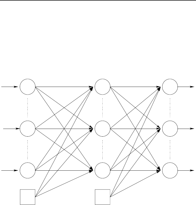
28 3. Supervised Learning Neural Networks

3.1.1 Feedforward Neural Networks

Figure 3.1 illustrates a standard feedforward neural network (FFNN), consisting of

three layers: an input layer (note that some literature on NNs do not count the input

layer as a layer), a hidden layer and an output layer. While this ﬁgure illustrates

only one hidden layer, a FFNN can have more than one hidden layer. However, it

has been proved that FFNNs with monotonically increasing diﬀerentiable functions

can approximate any continuous function with one hidden layer, provided that the

hidden layer has enough hidden neurons [383]. A FFNN can also have direct (linear)

connections between the input layer and the output layer.

−1−1

I+1

J+1

J,I +1

K,J+1

J+1,k

I+1,j

Figure 3.1 Feedforward Neural Network

The output of a FFNN for any given input pattern z

is calculated with a single

forward pass through the network. For each output unit o

, we have (assuming no

direct connections between the input and output layers),

k,p

= f

(net

k,p

)

= f





J+1



j=1

(net

j,p

)





= f





J+1



j=1



I+1



i=1

i,p







(3.1)

where f

and f

are respectively the activation function for output unit o

and

3.1 Neural Network Types 29

hidden unit y

; w

is the weight between output unit o

and hidden unit y

; z

i,p

is the value of input unit z

of input pattern z

;the(I + 1)-th input unit and the

(J + 1)-th hidden unit are bias units representing the threshold values of neurons in

the next layer.

Note that each activation function can be a diﬀerent function. It is not necessary that

all activation functions be the same. Also, each input unit can implement an activation

function. It is usually assumed that input units have linear activation functions.

−1

J+1

K,J+1

J+1,k

L−1

−1

J,L+1

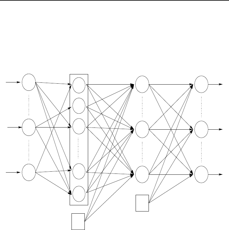
Figure 3.2 Functional Link Neural Network

3.1.2 Functional Link Neural Networks

In functional link neural networks (FLNN) input units do implement activation func-

tions (or rather, transformation functions). A FLNN is simply a FFNN with the input

layer expanded into a layer of functional higher-order units [314, 401]. The input layer,

with dimension I, is therefore expanded to functional units h

, ···,h

, where L is

the total number of functional units, and each functional unit h

is a function of the

input parameter vector (z

, ···,z

), i.e. h

, ···,z

) (see Figure 3.2). The weight

matrix U between the input layer and the layer of functional units is deﬁned as



1 if functional unit h

is dependent of z

0otherwise

(3.2)

For FLNNs, v

is the weight between hidden unit y

and functional link h

30 3. Supervised Learning Neural Networks

Calculation of the activation of each output unit o

occurs in the same manner as for

FFNNs, except that the additional layer of functional units is taken into account:

k,p

= f





J+1



j=1





l=1

)







(3.3)

The use of higher-order combinations of input units may result in faster training times

and improved accuracy (see, for example, [314, 401]).

3.1.3 Product Unit Neural Networks

Product unit neural networks (PUNN) have neurons that compute the weighted prod-

uct of input signals, instead of a weighted sum [222, 412, 509]. For product units, the

net input is computed as given in equation (2.5).

Diﬀerent PUNNs have been suggested. In one type each input unit is connected to

SUs, and to a dedicated group of PUs. Another PUNN type has alternating layers of

product and summation units. Due to the mathematical complexity of having PUs

in more than one hidden layer, this section only illustrates the case for which just

the hidden layer has PUs, and no SUs. The output layer has only SUs, and linear

activation functions are assumed for all neurons in the network. Then, for each hidden

unit y

, the net input to that hidden unit is (note that no bias is included)

net

j,p



i=1

i,p



i=1

ln(z

i,p

)

= e



ln(z

i,p

)

(3.4)

where z

i,p

is the activation value of input unit z

,andv

is the weight between input

and hidden unit y

An alternative to the above formulation of the net input signal for PUs is to include

a “distortion” factor within the product [406], such as

net

j,p

I+1



i=1

i,p

(3.5)

where z

I+1,p

= −1 for all patterns; v

j,I+1

represents the distortion factor. The purpose

of the distortion factor is to dynamically shape the activation function during training

to more closely ﬁt the shape of the true function represented by the training data.

If z

i,p

< 0, then z

i,p

can be written as the complex number z

i,p

= ı

i,p

| (ı =

√

−1)

that, substituted in (3.4), yields

net

j,p

= e



ln |z

i,p



ln ı

(3.6)

3.1 Neural Network Types 31

Let c =0+ı = a + bı be a complex number representing ı. Then,

ln c =lnre

ıθ

=lnr + ıθ +2πkı (3.7)

where r =

√

+ b

=1.

Considering only the main argument, arg(c), k = 0 which implies that 2πkı =0.

Furthermore, θ =

for ı =(0, 1). Therefore, ıθ = ı

, which simpliﬁes equation (3.10)

to ln c = ı

, and consequently,

ln ı

= ıπ (3.8)

Substitution of (3.8) in (3.6) gives

net

j,p

= e



ln |z

i,p



πı

= e



ln |z

i,p



cos(



i=1

π)+ı sin





i=1



(3.9)

Leaving out the imaginary part ([222] show that the added complexity of including

the imaginary part does not help with increasing performance),

net

j,p

= e



ln |z

i,p

cos





i=1



(3.10)

Now, let

j,p



i=1

ln |z

i,p

| (3.11)

j,p



i=1

(3.12)

with



0ifz

i,p

> 0

1ifz

i,p

< 0

(3.13)

and z

i,p

=0.

Then,

net

j,p

= e

j,p

cos(πφ

j,p

) (3.14)

The output value for each output unit is then calculated as

k,p

= f





J+1



j=1

j,p

cos(πφ

j,p

))





(3.15)

Note that a bias is now included for each output unit.

32 3. Supervised Learning Neural Networks

3.1.4 Simple Recurrent Neural Networks

Simple recurrent neural networks (SRNN) have feedback connections which add the

ability to also learn the temporal characteristics of the data set. Several diﬀerent types

of SRNNs have been developed, of which the Elman and Jordan SRNNs are simple

extensions of FFNNs.

Ŧ1

Context layer

Figure 3.3 Elman Simple Recurrent Neural Network

The Elman SRNN [236], as illustrated in Figure 3.3, makes a copy of the hidden

layer, which is referred to as the context layer. The purpose of the context layer is to

store the previous state of the hidden layer, i.e. the state of the hidden layer at the

previous pattern presentation. The context layer serves as an extension of the input

layer, feeding signals representing previous network states, to the hidden layer. The

input vector is therefore

z =(z

, ···,z

I+1

  

actual inputs

I+2

, ···,z

I+1+J

  

context units

) (3.16)

Context units z

I+2

, ···,z

I+1+J

are fully interconnected with all hidden units. The

connections from each hidden unit y

(for j =1, ···,J) to its corresponding context

3.1 Neural Network Types 33

unit z

I+1+j

have a weight of 1. Hence, the activation value y

is simply copied to

I+1+j

. It is, however, possible to have weights not equal to 1, in which case the

inﬂuence of previous states is weighted. Determining such weights adds additional

complexity to the training step.

Each output unit’s activation is then calculated as

k,p

= f





J+1



j=1

(

I+1+J



i=1

i,p

)





(3.17)

where (z

I+2,p

, ···,z

I+1+J,p

)=(y

1,p

(t − 1), ···,y

J,p

(t − 1)).

Ŧ1

State layer

Figure 3.4 Jordan Simple Recurrent Neural Network

Jordan SRNNs [428], on the other hand, make a copy of the output layer instead of

the hidden layer. The copy of the output layer, referred to as the state layer, extends

the input layer to

z =(z

, ···,z

I+1

  

actual inputs

I+2

, ···,z

I+1+K

  

state units

) (3.18)

The previous state of the output layer then also serves as input to the network. For

34 3. Supervised Learning Neural Networks

each output unit,

k,p

= f





J+1



j=1



I+1+K



i=1

i,p







(3.19)

where (z

I+2,p

, ···,z

I+1+K,p

)=(o

1,p

(t − 1), ···,o

K,p

(t − 1)).

Ŧ1

(t)

j,1(t)

j,1(t−1)

j,1(t−2)

j,1(t−n

)

j,2(t)

j,2(t−1)

j,2(t−2)

j,2(t−n

)

j,I(t)

j,I(t−1)

j,I(t−2)

j,I(t−n

)

j,I+1

(t − 1)

(t − 2)

(t − n

)

(t − n

)

(t − 2)

(t − 1)

(t − n

)

(t − 2)

(t − 1)

Figure 3.5 A Single Time-Delay Neuron

3.1.5 Time-Delay Neural Networks

A time-delay neural network (TDNN) [501], also referred to as backpropagation-

through-time, is a temporal network with its input patterns successively delayed in

3.1 Neural Network Types 35

time. A single neuron with n

time delays for each input unit is illustrated in Fig-

ure 3.5. This type of neuron is then used as a building block to construct a complete

feedforward TDNN.

Initially, only z

i,p

(t), with t = 0, has a value and z

i,p

(t −t



) is zero for all i =1, ···,I

with time steps t



=1, ···,n

; n

is the total number of time steps, or number of delayed

patterns. Immediately after the ﬁrst pattern is presented, and before presentation of

the second pattern,

i,p

(t − 1) = z

i,p

(t) (3.20)

After presentation of t



patterns and before the presentation of pattern t



+ 1, for all

t =1, ···,t



i,p

(t − t



)=z

i,p

(t − t



+ 1) (3.21)

This causes a total of n

patterns to inﬂuence the updates of weight values, thus

allowing the temporal characteristics to drive the shaping of the learned function.

Each connection between z

i,p

(t − t



)andz

i,p

(t − t



+ 1) has a value of 1.

The output of a TDNN is calculated as

k,p

= f





J+1



j=1





i=1



t=0

j,i(t)

i,p

(t)+z

I+1

j,I+1







(3.22)

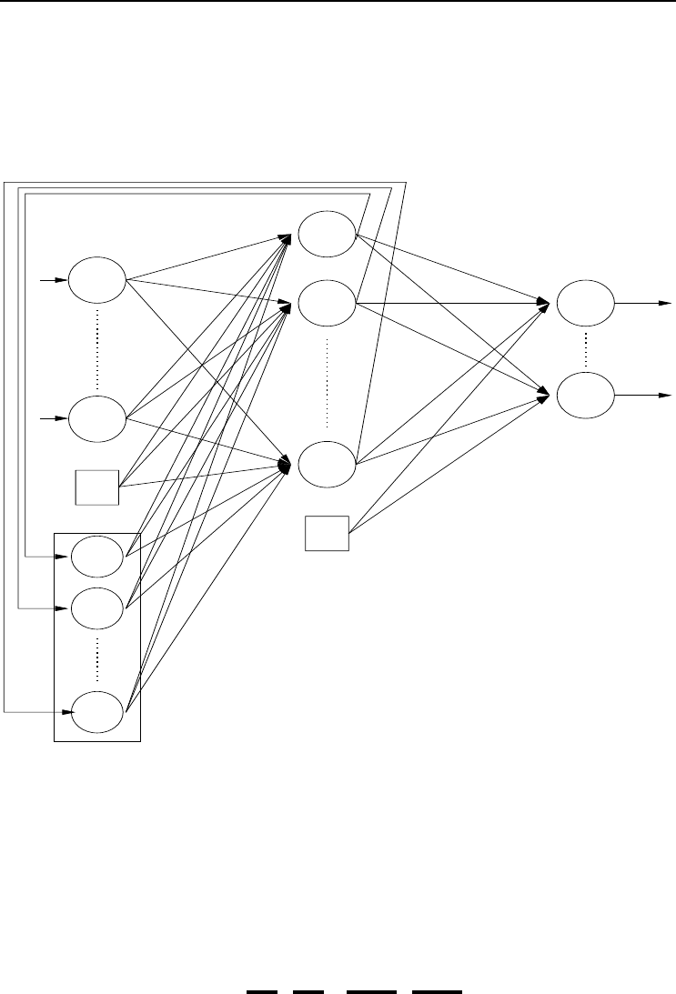
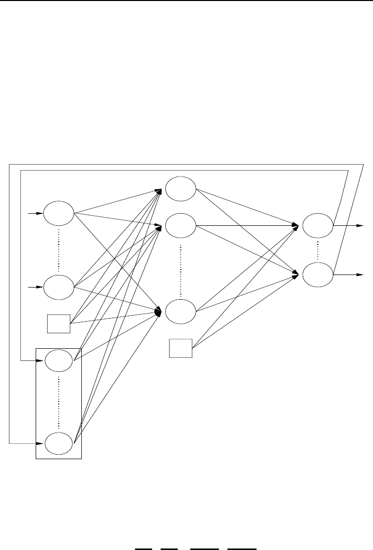
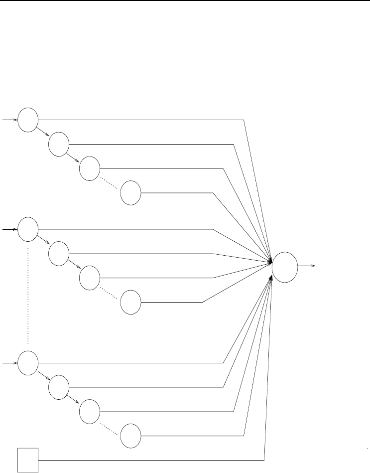
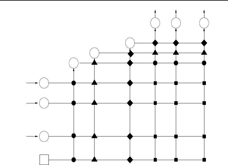
3.1.6 Cascade Networks

A cascade NN (CNN) [252, 688] is a multilayer FFNN where all input units have direct

connections to all hidden units and to all output units. Furthermore, the hidden units

are cascaded. That is, each hidden unit’s output serves as an input to all succeeding

hidden units and all output units. Figure 3.6 illustrates a CNN.

The output of a CNN is calculated is

k,p

= f





I+1



i=1



j=1



I+1



i=1

j−1



l=1







(3.23)

where u

represents a weight between output unit k and input unit i, s

is a weight

between hidden units j and l,andy

is the activation of hidden unit l.

At this point it is important to note that training of a CNN consists of ﬁnding weight

values and the size of the NN. Training starts with the simplest architecture containing

only the (I +1)K direct weights between input and output units (indicated by a solid

square in Figure 3.6). If the accuracy of the CNN is unacceptable one hidden unit

is added, which adds another (I +1)J +(J − 1) + JK weights to the network. If

J = 1, the network includes the weights indicated by the ﬁlled squares and circles in

Figure 3.6. When J = 2, the weights marked by ﬁlled triangles are added.

36 3. Supervised Learning Neural Networks

Ŧ1

I+1

Figure 3.6 Cascade Neural Network

3.2 Supervised Learning Rules

Up to this point it was shown how NNs can be used to calculate an output value given

an input pattern. This section explains approaches to train the NN such that the

output of the network is an accurate approximation of the target values. First, the

learning problem is explained, and then diﬀerent training algorithms are described.

3.2.1 The Supervised Learning Problem

Consider a ﬁnite set of input-target pairs D = {d

=(z

, t

)|p =1, ···,P} sampled

from a stationary density Ω(D), with z

i,p

k,p

∈ R for i =1, ···,I and k =1, ···,K;

i,p

is the value of input unit z

and t

k,p

is the target value of output unit o

for

pattern p. According to the signal-plus-noise model,

= µ(z

)+ζ

(3.24)

where µ(z) is the unknown function. The input values z

i,p

are sampled with probability

density ω(z), and the ζ

k,p

are independent, identically distributed noise sampled with

density φ(ζ), having zero mean. The objective of learning is then to approximate the

unknown function µ(z) using the information contained in the ﬁnite data set D.For

NN learning this is achieved by dividing the set D randomly into a training set D

a validation set D

, and a test set D

(all being dependent from one another). The

3.2 Supervised Learning Rules 37

approximation to µ(z) is found from the training set D

, memorization is determined

from D

(more about this later), and the generalization accuracy is estimated from

the test set D

(more about this later).

Since prior knowledge about Ω(D) is usually not known, a nonparametric regression

approach is used by the NN learner to search through its hypothesis space H for a

function f

, W) which gives a good estimation of the unknown function µ(z),

where f

, W) ∈H. For multilayer NNs, the hypothesis space consists of all

functions realizable from the given network architecture as described by the weight

vector W .

During learning, the function f

: R

−→ R

is found which minimizes the empirical

error

; W)=



p=1

, W) − t

)

(3.25)

where P

is the total number of training patterns. The hope is that a small empirical

(training) error will also give a small true error, or generalization error, deﬁned as

(Ω; W)=



(z, W) − t)

dΩ(z, t) (3.26)

For the purpose of NN learning, the empirical error in equation (3.25) is referred

to as the objective function to be optimized by the optimization method. Several

optimization algorithms for training NNs have been developed [51, 57, 221]. These

algorithms are grouped into two classes:

• Local optimization, where the algorithm may get stuck in a local optimum

without ﬁnding a global optimum. Gradient descent and scaled conjugate gra-

dient are examples of local optimizers.

• Global optimization, where the algorithm searches for the global optimum

by employing mechanisms to search larger parts of the search space. Global

optimizers include LeapFrog, simulated annealing, evolutionary algorithms and

swarm optimization.

Local and global optimization techniques can be combined to form hybrid training

algorithms.

Learning consists of adjusting weights until an acceptable empirical error has been

reached. Two types of supervised learning algorithms exist, based on when weights

are updated:

• Stochastic/online learning, where weights are adjusted after each pattern

presentation. In this case the next input pattern is selected randomly from

the training set, to prevent any bias that may occur due to the order in which

patterns occur in the training set.

• Batch/offline learning, where weight changes are accumulated and used to

adjust weights only after all training patterns have been presented.