Engelbrecht Andries P. Computational Intelligence: An Introduction

Подождите немного. Документ загружается.

238 13. Differential Evolution

parameters are discussed in Section 13.1.6. A geometric illustration of the DE variation

approach is given in Section 13.1.7.

13.1.1 Diﬀerence Vectors

The positions of individuals provide valuable information about the ﬁtness landscape.

Provided that a good uniform random initialization method is used to construct the

initial population, the initial individuals will provide a good representation of the

entire search space, with relatively large distances between individuals. Over time,

as the search progresses, the distances between individuals become smaller, with all

individuals converging to the same solution. Keep in mind that the magnitude of the

initial distances between individuals is inﬂuenced by the size of the population. The

more individuals in a population, the smaller the magnitude of the distances.

Distances between individuals are a very good indication of the diversity of the current

population, and of the order of magnitude of the step sizes that should be taken

in order for the population to contract to one point. If there are large distances

between individuals, it stands to reason that individuals should make large step sizes

in order to explore as much of the search space as possible. On the other hand,

if the distances between individuals are small, step sizes should be small to exploit

local areas. It is this behaviour that is achieved by DE in calculating mutation step

sizes as weighted diﬀerences between randomly selected individuals. The ﬁrst step of

mutation is therefore to ﬁrst calculate one or more diﬀerence vectors, and then to use

these diﬀerence vectors to determine the magnitude and direction of step sizes.

Using vector diﬀerentials to achieve variation has a number of advantages. Firstly,

information about the ﬁtness landscape, as represented by the current population, is

used to direct the search. Secondly, due to the central limit theorem [177], mutation

step sizes approaches a Gaussian (Normal) distribution, provided that the population

is suﬃciently large to allow for a good number of diﬀerence vectors [811].

The mean

of the distribution formed by the diﬀerence vectors are always zero, provided that

individuals used to calculate diﬀerence vectors are selected uniformly from the pop-

ulation [695, 164]. Under the condition that individuals are uniformly selected, this

characteristic follows from the fact that diﬀerence vectors (x

− x

)and(x

− x

)

occur with equal frequency, where x

and x

are two randomly selected individuals.

The zero mean of the resulting step sizes ensures that the population will not suﬀer

from genetic drift. It should also be noted that the deviation of this distribution is

determined by the magnitude of the diﬀerence vectors. Eventually, diﬀerentials will

become inﬁnitesimal, resulting in very small mutations.

Section 13.2 shows that more than one diﬀerential can be used to determine the muta-

tion step size. If n

is the number of diﬀerentials used, and n

is the population size,

then the total number of diﬀerential perturbations is given by [429]





! ≈O(n

) (13.1)

The central limit theorem states that the probability distribution governing a random variable

approaches the Normal distribution as the number of samples of that random variable tends to inﬁnity.

13.1 Basic Differential Evolution 239

Equation (13.1) expresses the total number of directions that can be explored per

generation. To increase the exploration power of DE, the number of directions can be

increased by increasing the population size and/or the number of diﬀerentials used.

At this point it is important to emphasize that the original DE was developed for

searching through continuous-valued landscapes. The sections that follow will show

that exploration of the search space is achieved using vector algebra, applied to the

individuals of the current population.

13.1.2 Mutation

The DE mutation operator produces a trial vector for each individual of the current

population by mutating a target vector with a weighted diﬀerential. This trial vector

will then be used by the crossover operator to produce oﬀspring. For each parent,

(t), generate the trial vector, u

(t), as follows: Select a target vector, x

(t), from

the population, such that i = i

. Then, randomly select two individuals, x

and x

from the population such that i = i

= i

and i

∼ U(1,n

). Using these

individuals, the trial vector is calculated by perturbing the target vector as follows:

(t)=x

(t)+β(x

(t) − x

(t)) (13.2)

where β ∈ (0, ∞) is the scale factor, controlling the amplication of the diﬀerential

variation.

Diﬀerent approaches can be used to select the target vector and to calculate diﬀeren-

tials as discussed in Section 13.2.

13.1.3 Crossover

The DE crossover operator implements a discrete recombination of the trial vector,

(t), and the parent vector, x

(t), to produce oﬀspring, x



(t). Crossover is imple-

mented as follows:



(t)=



(t)ifj ∈J

(t)otherwise

(13.3)

where x

(t) refers to the j-th element of the vector x

(t), and J is the set of element

indices that will undergo perturbation (or in other words, the set of crossover points).

Diﬀerent methods can be used to determine the set, J, of which the following two

approaches are the most frequently used [811, 813]:

• Binomial crossover: The crossover points are randomly selected from the set

of possible crossover points, {1, 2,...,n

},wheren

is the problem dimension.

Algorithm 13.1 summarizes this process. In this algorithm, p

is the probability

that the considered crossover point will be included. The larger the value of

, the more crossover points will be selected compared to a smaller value. This

means that more elements of the trial vector will be used to produce the oﬀspring,

and less of the parent vector. Because a probabilistic decision is made as to the

240 13. Differential Evolution

inclusion of a crossover point, it may happen that no points may be selected, in

which case the oﬀspring will simply be the original parent, x

(t). This problem

becomes more evident for low dimensional search spaces. To enforce that at least

one element of the oﬀspring diﬀers from the parent, the set of crossover points,

J, is initialized to include a randomly selected point, j

∗

• Exponential crossover: From a randomly selected index, the exponential

crossover operator selects a sequence of adjacent crossover points, treating the

list of potential crossover points as a circular array. The pseudocode in Algo-

rithm 13.2 shows that at least one crossover point is selected, and from this

index, selects the next until U(0, 1) ≥ p

or |J| = n

Algorithm 13.1 Diﬀerential Evolution Binomial Crossover for Selecting Crossover

Points

∗

∼ U(1,n

);

J←J∪{j

∗

};

for each j ∈{1,...,n

} do

if U(0, 1) <p

and j = j

∗

then

J←J∪{j};

end

Algorithm 13.2 Diﬀerential Evolution Exponential Crossover for Selecting Crossover

Points

J←{};

j ∼ U(0,n

− 1);

repeat

J←J∪{j +1};

j =(j +1)modn

;

until U(0, 1) ≥ p

or |J| = n

;

13.1.4 Selection

Selection is applied to determine which individuals will take part in the mutation

operation to produce a trial vector, and to determine which of the parent or the

oﬀspring will survive to the next generation. With reference to the mutation operator,

a number of selection methods have been used. Random selection is usually used

to select the individuals from which diﬀerence vectors are calculated. For most DE

implementations the target vector is either randomly selected or the best individual is

selected (refer to Section 13.2).

To construct the population for the next generation, deterministic selection is used:

the oﬀspring replaces the parent if the ﬁtness of the oﬀspring is better than its parent;

otherwise the parent survives to the next generation. This ensures that the average

ﬁtness of the population does not deteriorate.

13.1 Basic Differential Evolution 241

13.1.5 General Diﬀerential Evolution Algorithm

Algorithm 13.3 provides a generic implementation of the basic DE strategies. Initial-

ization of the population is done by selecting random values for the elements of each

individual from the bounds deﬁned for the problem being solved. That is, for each

individual, x

(t), x

(t) ∼ U(x

min,j

max,j

), where x

min

and x

max

deﬁne the search

boundaries.

Any of the stopping conditions given in Section 8.7 can be used to terminate the

algorithm.

Algorithm 13.3 General Diﬀerential Evolution Algorithm

Set the generation counter, t =0;

Initialize the control parameters, β and p

;

Create and initialize the population, C(0), of n

individuals;

while stopping condition(s) not true do

for each individual, x

(t) ∈C(t) do

Evaluate the ﬁtness, f(x

(t));

Create the trial vector, u

(t) by applying the mutation operator;

Create an oﬀspring, x



(t), by applying the crossover operator;

if f(x



(t)) is better than f(x

(t)) then

Add x



(t)toC(t +1);

end

else

Add x

(t)toC(t +1);

end

Return the individual with the best ﬁtness as the solution;

13.1.6 Control Parameters

In addition to the population size, n

, the performance of DE is inﬂuenced by two

control parameters, the scale factor, β, and the probability of recombination, p

.The

eﬀects of these parameters are discussed below:

• Population size: As indicated in equation (13.1), the size of the population

has a direct inﬂuence on the exploration ability of DE algorithms. The more

individuals there are in the population, the more diﬀerential vectors are available,

and the more directions can be explored. However, it should be kept in mind

that the computational complexity per generation increases with the size of the

population. Empirical studies provide the guideline that n

≈ 10n

. The nature

of the mutation process does, however, provide a lower bound on the number of

individuals as n

> 2n

+1, where n

is the number of diﬀerentials used. For n

diﬀerentials, 2n

diﬀerent individuals are required, 2 for each diﬀerential. The

242 13. Differential Evolution

additional individual represents the target vector.

• Scaling factor: The scaling factor, β ∈ (0, ∞), controls the ampliﬁcation of the

diﬀerential variations, (x

−x

). The smaller the value of β, the smaller the mu-

tation step sizes, and the longer it will be for the algorithm to converge. Larger

values for β facilitate exploration, but may cause the algorithm to overshoot

good optima. The value of β should be small enough to allow diﬀerentials to

explore tight valleys, and large enough to maintain diversity. As the population

size increases, the scaling factor should decrease. As explained in Section 13.1.1,

the more individuals in the population, the smaller the magnitude of the dif-

ference vectors, and the closer individuals will be to one another. Therefore,

smaller step sizes can be used to explore local areas. More individuals reduce

the need for large mutation step sizes. Empirical results suggest that large val-

ues for both n

and β often result in premature convergence [429, 124], and that

β =0.5 generally provides good performance [813, 164, 19].

• Recombination probability: The probability of recombination, p

,hasadi-

rect inﬂuence on the diversity of DE. This parameter controls the number of

elements of the parent, x

(t), that will change. The higher the probability of

recombination, the more variation is introduced in the new population, thereby

increasing diversity and increasing exploration. Increasing p

often results in

faster convergence, while decreasing p

increases search robustness [429, 164].

Most implementations of DE strategies keep the control parameters constant. Al-

though empirical results have shown that DE convergence is relatively insensitive to

diﬀerent values of these parameters, performance (in terms of accuracy, robustnes, and

speed) can be improved by ﬁnding the best values for control parameters for each new

problem. Finding optimal parameter values can be a time consuming exercise, and

for this reason, self-adaptive DE strategies have been developed. These methods are

discussed in Section 13.3.3.

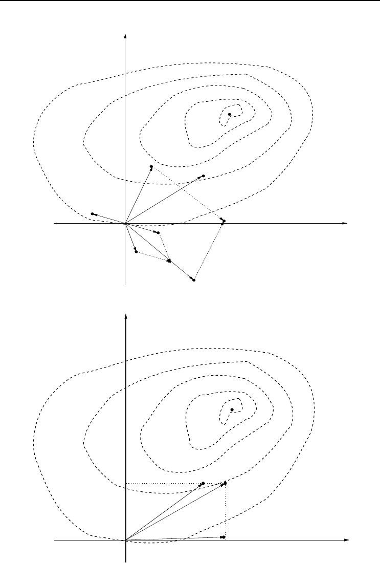
13.1.7 Geometrical Illustration

Figure 13.1(a) illustrates the mutation operator of the DE as described in Sec-

tion 13.1.2. The optimum is indicated by x

∗

, and it is assumed that β =1.5. The

crossover operator is illustrated in Figure 13.1(b). For this illustration the oﬀspring

consists of the ﬁrst element of the trial vector, u

(t), and the second element of the

parent, x

(t).

13.2 DE/x/y/z

A number of variations to the basic DE as discussed in Section 13.1 have been devel-

oped. The diﬀerent DE strategies diﬀer in the way that the target vector is selected,

the number of diﬀerence vectors used, and the way that crossover points are deter-

mined. In order to characterize these variations, a general notation was adopted in

the DE literature, namely DE/x/y/z [811, 813]. Using this notation, x refers to the

13.2 DE/x/y/z 243

∗

(t)

−x

(t)

β(x

(t) −x

(t))

(t)

(t) −x

(t)

(a) Mutation Operator

∗

(t)



(t)

(b) Crossover Operator

Figure 13.1 Diﬀerential Evolution Mutation and Crossover Illustrated

244 13. Differential Evolution

method of selecting the target vector, y indicates the number of diﬀerence vectors

used, and z indicates the crossover method used. The DE strategy discussed in Sec-

tion 13.1 is referred to as DE/rand/1/bin for binomial crossover, and DE/rand/1/exp

for exponential crossover. Other basic DE strategies include [429, 811, 813]:

• DE/best/1/z: For this strategy, the target vector is selected as the best in-

dividual,

x(t), from the current population. In this case, the trial vector is

calculated as

(t)=

x(t)+β(x

(t) − x

(t)) (13.4)

Any of the crossover methods can be used.

• DE/x/n

/z: For this strategy, more than one diﬀerence vector is used. The

trial vector is calculated as

(t)=x

(t)+β



k=1

(t) − x

(t)) (13.5)

where x

(t)−x

(t) indicates the k-th diﬀerence vector, x

(t) can be selected

using any suitable method for selecting the target vector, and any of the crossover

methods can be used. With reference to equation (13.1), the larger the value of

, the more directions can be explored per generation.

• DE/rand-to-best/n

/z: This strategy combines the rand and best strategies

to calculate the trial vector as follows:

(t)=γ

x(t)+(1− γ)x

(t)+β



k=1

(t) − x

(t)) (13.6)

where x

(t) is randomly selected, and γ ∈ [0, 1] controls the greediness of the

mutation operator. The closer γ is to 1, the more greedy the search process

becomes. In other words, γ close to 1 favors exploitation while a value close to 0

favors exploration. A good strategy will be to use an adaptive γ,withγ(0) = 0.

The value of γ(t) increases with each new generation towards the value 1.

Note that if γ = 0, the DE/rand/y/z strategies are obtained, while γ =1gives

the DE/best/y/z strategies.

• DE/current-to-best/1+n

/z: With this strategy, the parent is mutated using

at least two diﬀerence vectors. One diﬀerence vector is calculated from the best

vector and the parent vector, while the rest of the diﬀerence vectors are calculated

using randomly selected vectors:

(t)=x

(t)+β(

x(t) − x

(t)) + β



k=1

(t) − x

(t)) (13.7)

Empirical studies have shown that DE/rand/1/bin maintains good diversity, while

DE/current-to-best/2/bin shows good convergence characteristics [698]. Due to this

observation, Qin and Suganthan [698] developed a DE algorithm that dynamically

switch between these two strategies. Each of these strategies is assigned a probability

13.3 Variations to Basic Differential Evolution 245

of being applied. If p

s,1

is the probability that DE/rand/1/bin will be applied, then

s,2

=1−p

s,1

is the probability that DE/current-to-best/2/bin will be applied. Then,

s,1

s,2

+ n

f,2

)

s,2

s,1

+ n

f,1

)+n

s,1

s,2

+ n

f,2

)

(13.8)

where n

s,1

and n

s,2

are respectively the number of oﬀspring that survive to the next

generation for DE/rand/1/bin, and n

f,1

and n

f,2

represent the number of discarded

oﬀspring for each strategy. The more oﬀspring that survive for a speciﬁc strategy, the

higher the probability for selecting that strategy for the next generation.

13.3 Variations to Basic Diﬀerential Evolution

The basic DE strategies have been shown to be very eﬃcient and robust [811, 813,

811, 813]. A number of adaptations of the original DE strategies have been developed

in order to further improve performance. This section reviews some of these DE varia-

tions. Section 13.3.1 describe hybrid DE methods, a population-based DE is described

in Section 13.3.2, and self-adaptive DE strategies are discussed in Section 13.3.3.

13.3.1 Hybrid Diﬀerential Evolution Strategies

DE has been combined with other EAs, particle swarm optimization (PSO), and

gradient-based techniques. This section summarizes some of these hybrid methods.

Gradient-Based Hybrid Diﬀerential Evolution

One of the ﬁrst DE hybrids was developed by Chiou and Wang [124], referred to

as the hybrid DE. As indicated in Algorithm 13.4, the hybrid DE introduces two

new operations: an acceleration operator to improve convergence speed – without

decreasing diversity – and a migration operator to provide the DE with the improved

ability to escape local optima.

The acceleration operator uses gradient descent to adjust the best individual toward

obtaining a better position if the mutation and crossover operators failed to improve

the ﬁtness of the best individual. Let

x(t) denote the best individual of the current

population, C(t), before application of the mutation and crossover operators, and let

x(t + 1) be the best individual for the next population after mutation and crossover

have been applied to all individuals. Then, assuming a minimization problem, the

acceleration operator computes the vector

x(t)=



x(t +1) if f (

x(t +1))<f(

x(t))

x(t +1)− η(t)∇f otherwise

(13.9)

where η(t) ∈ (0, 1] is the learning rate, or step size; ∇f is the gradient of the objective

function, f . The new vector, x(t), replaces the worst individual in the new population,

C(t).

246 13. Differential Evolution

Algorithm 13.4 Hybrid Diﬀerential Evolution with Acceleration and Migration

Set the generation counter, t =0;

Initialize the control parameters, β and p

;

Create and initialize the population, C(0), of n

individuals;

while stopping condition(s) not true do

Apply the migration operator if necessary;

for each individual, x

(t) ∈C(t) do

Evaluate the ﬁtness, f(x

(t));

Create the trial vector, u

(t) by applying the mutation operator;

Create an oﬀspring, x



(t) by applying the crossover operator;

if f(x



(t)) is better than f(x

(t)) then

Add x



(t)toC(t +1);

end

else

Add x

(t)toC(t +1);

end

Apply the acceleration operator if necessary;

end

Return the individual with the best ﬁtness as the solution;

The learning rate is initialized to one, i.e. η(0) = 1. If the gradient descent step failed

to create a new vector, x(t), with better ﬁtness, the learning rate is reduced by a

factor. The gradient descent step is then repeated until η(t)∇f is suﬃciently close to

zero, or a maximum number of gradient descent steps have been executed.

While use of gradient descent can signiﬁcantly speed up the search, it has the disad-

vantage that the DE may get stuck in a local minimum, or prematurely converge. The

migration operator addresses this problem by increasing population diversity. This is

done by spawning new individuals from the best individual, and replacing the current

population with these new individuals. Individuals are spawned as follows:



(t)=

ˆx

(t)+r

min,j

− ˆx

)ifU (0, 1) <

ˆx

−x

min,j

max,j

−x

min,j

ˆx

(t)+r

max,j

− ˆx

)otherwise

(13.10)

where r

∼ U(0, 1). Spawned individual x



(t) becomes x

(t +1).

The migration operator is applied only when the diversity of the current population

becomes too small; that is, when









i=1

(t)=

x(t)

(t)







/(n

− 1)) <

(13.11)

13.3 Variations to Basic Differential Evolution 247

with

(t)=



1if|(x

(t) − ˆx

(t))/ˆx

(t)| >

0otherwise

(13.12)

where 

and 

are respectively the tolerance for the population diversity and gene

diversity with respect to the best individual,

x(t). If I

(t) = 0, then the value of

the j-th element of individual i is close to the value of the j-th element of the best

individual.

Magoulas et al. [550] combined a stochastic gradient descent (SGD) [549] and DE in

a sequential manner to train artiﬁcial neural networks (NN). Here, SGD is ﬁrst used

to ﬁnd a good approximate solution using the process outlined in Algorithm 13.5. A

population of DE individuals is then created, with individuals in the neighborhood of

the solution returned by the SGD step. As outlined in Algorithm 13.6, the task of

DE is to reﬁne the solution obtained from SGD by using then DE to perform a local

search.

Algorithm 13.5 Stochastic Gradient Descent for Neural Network Training

Initialize the NN weight vector, w(0);

Initialize the learning rate, η(0), and the meta-step size, η

;

Set the pattern presentation number, t =0;

repeat

for each training pattern, p do

Calculate E(w(t));

Calculate ∇E(w(t));

Update the weights using

w(t +1)=w(t)+η(t)∇E(w(t)) (13.13)

Calculate the new step size using

η(t +1)=η(t)+η

< ∇E(w(t − 1)), ∇E(w(t)) > (13.14)

t = t +1;

end

Return w(t + 1) as the solution;

until until a termination condition is satisfied;

In Algorithms 13.5 and 13.6, < •, • > denotes the inner product between the two

given vectors, E is the NN training objective function (usually the sum-squared error),

σ is the standard deviation of mutations to w used to create DE individuals in the

neighborhood of w,andD

is the training set. The DE algorithm uses the objective

function, E, to assess the ﬁtness of individuals.