Enns R.H. Computer Algebra Recipes for Mathematical Physics
Подождите немного. Документ загружается.


3.3. MATRICES 117
Provided that non-zero values are chosen for the undetermined elements, the
inverse matrix C
−1
exists. Now we calculate C
−1
AC, obtaining the diagonal
matrix S as expected.
>
check:=Cinverse . (A . C);
check :=
⎡
⎣
−20 0
09 0
00−18
⎤
⎦
A particular matrix C which will accomplish the transformation is now obtained
by setting all the undetermined matrix elements equal to 1.
>
C:=eval(C,{c[2,1]=1,c[3,2]=1,c[2,3]=1});
C :=
⎡
⎣
−1 −21
1 −21
014
⎤
⎦
3.3.4 Orthogonal and Unitary Matrices
No matter how calmly you try to referee, parenting will eventually
produce bizarre behavior, and I’m not talking about the kids. Their
behavior is always normal.
Bill Cosby, American comedian, Fatherhood, 1986
The ideas of orthogonality and normalization which are important in the discus-
sion of vectors can be extended to matrices as illustrated in this simple recipe.
(a) If A =
⎛
⎝
a1
a2
a3
⎞
⎠
,B=
⎛
⎝
b1
b2
b3
⎞
⎠
,C=
⎛
⎝
c1
c2
c3
⎞
⎠
are real mutually orthogonal unit column vectors, prove that the real matrix
ABC =
⎛
⎝
a1 b1 c1
a2 b2 c2
a3 b3 c3
⎞
⎠
is an orthogonal matrix. A real matrix M is referred to as an orthogonal matrix
if its transpose is equal to its inverse, i.e., M
T
=M
−1
,orM
T
M =I.
(b) With i=
√
−1, show that
H =
⎛
⎜
⎜
⎜
⎜
⎜
⎝
√
2
2
−i
√
2
2
0
i
√
2
2
−
√
2
2
0
001
⎞
⎟
⎟
⎟
⎟
⎟
⎠
is a unitary matrix. A complex matrix M is a unitary matrix if its complex
conjugate transpose is equal to its inverse, i.e., (M
∗
)
T
=M
−1
,or(M
∗
)
T
M =I.

118 CHAPTER 3. VECTORS AND MATRICES
After the usual loading of the LinearAlgebra package when dealing with ma-
trices, the column vectors A, B,andC are entered using the Vector command,
each argument containing a list of the relevant elements.
>
restart: with(LinearAlgebra):
>
A:=Vector([a1,a2,a3]); B:=Vector([b1,b2,b3]);
C:=Vector([c1,c2,c3]);
A :=
⎡
⎣
a1
a2
a3
⎤
⎦
B :=
⎡
⎣
b1
b2
b3
⎤
⎦
C :=
⎡
⎣
c1
c2
c3
⎤
⎦
A functional operator F is introduced for imposing “orthonormality” on arbi-
trary column vectors M and N. Normalization follows on setting the parameter
n= 1, orthogonality on setting n=0.
>
F:=(M,N,n)->(Transpose(M) . N)=n:
Using F, normalization is imposed on A, B,andC in eq1 , eq2 ,andeq3 ,and
orthogonality in eq4 , eq5 ,andeq6 .
>
eq||1:=F(A,A,1); eq||2:=F(B,B,1); eq||3:=F(C,C,1);
eq1 := a1
2
+ a2
2
+ a3
2
=1 eq2 := b1
2
+ b2
2
+ b3
2
=1
eq3 := c1
2
+ c2
2
+ c3
2
=1
>
eq||4:=F(A,B,0); eq||5:=F(A,C,0); eq||6:=F(B,C,0);
eq4 := b1 a1 + b2 a2 + b3 a3 =0 eq5 := c1 a1 + c2 a2 + c3 a3 =0
eq6 := c1 b1 + c2 b2 + c3 b3 =0
The matrix ABC is entered using the Matrix command.
>
ABC:=Matrix([[a1,b1,c1],[a2,b2,c2],[a3,b3,c3]]);
ABC :=
⎡
⎣
a1 b1 c1
a2 b2 c2
a3 b3 c3
⎤
⎦
To produce an orthogonal matrix OM , the product (ABC )
T
(ABC )isformed.
>
OM:=Transpose(ABC) . ABC;
OM :=
⎡
⎣
a1
2
+ a2
2
+ a3
2
, b1 a1 + b2 a2 + b3 a3 , c1 a1 + c2 a2 + c3 a3
b1 a1 + b2 a2 + b3 a3 , b1
2
+ b2
2
+ b3
2
, c1 b1 + c2 b2 + c3 b3
c1 a1 + c2 a2 + c3 a3 , c1 b1 + c2 b2 + c3 b3 , c1
2
+ c2
2
+ c3
2
⎤
⎦
Evaluating OM with the six orthonormality conditions, yields the identity
(unit) matrix, thus confirming that ABC is an orthogonal matrix.
>
OM2:=eval(OM,{seq(eq||i,i=1..6)});
OM2 :=
⎡
⎣
100
010
001
⎤
⎦
To answer part (b),theinterface(imaginaryunit=i) command is used to
set i ≡
√
−1. Then the matrix H is entered.
>
interface(imaginaryunit=i):

3.3. MATRICES 119
>
H:=<<sqrt(2)/2|-i*sqrt(2)/2|0>,<i*sqrt(2)/2|-sqrt(2)/2|0>,
<0|0|1>>;
H :=
⎡
⎢
⎢
⎢
⎢
⎢
⎣
√
2
2
−1
2
i
√
20
1
2
i
√
2 −
√
2
2
0
001
⎤
⎥
⎥
⎥
⎥
⎥
⎦
The HermitianTranspose command is applied to H in T . This command
applies the transpose (interchanging rows and columns) and takes the complex
conjugate of the elements.
>
T:=HermitianTranspose(H);
T :=
⎡
⎢
⎢
⎢
⎢
⎢
⎣
√
2
2
−1
2
i
√
20
1
2
i
√
2 −
√
2
2
0
001
⎤
⎥
⎥
⎥
⎥
⎥
⎦
Since T = H, H is a Hermitian matrix. That it is also a unitary matrix is
confirmed by forming the product HT, the result R being the unit matrix.
>
R:=H . T;
R :=
⎡
⎣
100
010
001
⎤
⎦
3.3.5 Introducing the Euler Angles
To knock a thing down, especially if it is cocked at an arrogant angle,
is a deep delight to the blood.
George Santayana, American philosopher (1863–1952)
The transformation from one 3-dimensional coordinate system (x, y, z)toan-
other (x
,y
,z
) with the same origin can be represented by a matrix equation
of the form X
=RX,whereR is the 3 × 3 rotation matrix and
X =
⎛
⎝
x
y
z
⎞
⎠
,X
=
⎛
⎝
x
y
z
⎞
⎠
.
The over-all rotation is made up of three 1-dimensional rotations through the
angles φ, θ,andψ, called the Euler angles. The choices of these angles is not
uniform in the literature
4
, so I will adopt the notation of Marion and Thornton
[MT95] and Goldstein, Poole, and Safco [GPS02].
4
In fact, Euler angles can be avoided altogether in classical physics by specifying a single
plane of rotation and one angle, as discussed for example in [Bay99], [DL03], and [Hes99].
120 CHAPTER 3. VECTORS AND MATRICES
The first rotation is counterclockwise through an angle φ about the z axis,
the rotation matrix being
R
φ
=
⎛
⎝
cos φ sin φ 0
−sin φ cos φ 0
001
⎞
⎠
.
The new axes are labeled x
1
, y
1
,andz
1
= z. The second rotation is coun-
terclockwise through an angle θ about the x
1
axis, the rotation matrix being
R
θ
=
⎛
⎝
10 0
0cosθ sin θ
0 −sin θ cos θ
⎞
⎠
.
The new axes are labeled x
2
=x
1
, y
2
, z
2
. The third rotation is counterclockwise
throughanangleψ about the z
2
axis, the rotation matrix being
R
φ
=
⎛
⎝
cos ψ sin ψ 0
−sin ψ cos ψ 0
001
⎞
⎠
.
The new axes are labeled x
, y
, z
= z
2
. The total rotation matrix then is
R= R
ψ
R
θ
R
φ
.
In this recipe, I will derive the total rotation matrix R and apply its inverse
to a triplet of vectors originally pointing along the x, y, z axes. The plots and
LinearAlgebra packages are first loaded.
>
restart: with(plots): with(LinearAlgebra):
To ease the typing, the aliases p, t,ands are introduced for the input quantities
phi, theta,andpsi.
>
alias(phi=p,theta=t,psi=s):
The three rotation matrices R
φ
, R
θ
,andR
ψ
are entered.
>
R[p]:=<<cos(p)|sin(p)|0>,<-sin(p)|cos(p)|0>,<0|0|1>>;
R
φ
:=
⎡
⎣
cos(φ)sin(φ)0
−sin(φ) cos(φ)0
001
⎤
⎦
>
R[t]:=<<1|0|0>,<0|cos(t)|sin(t)>,<0|-sin(t)|cos(t)>>;
R
θ
:=
⎡
⎣
10 0
0 cos(θ)sin(θ)
0 −sin(θ) cos(θ)
⎤
⎦
>
R[s]:=<<cos(s)|sin(s)|0>,<-sin(s)|cos(s)|0>,<0|0|1>>;
R
ψ
:=
⎡
⎣
cos(ψ)sin(ψ)0
−sin(ψ) cos(ψ)0
001
⎤
⎦
The total rotation matrix R= R
ψ
R
θ
R
φ
is then calculated.
>
R:=R[s] . (R[t] . R[p]);

3.3. MATRICES 121
R :=
⎡
⎣
cosψ cosφ −sinψ cosθ sinφ, cosψ sinφ +sinψ cosθ cosφ, sinψ sinθ
−sinψ cosφ −cosψ cosθ sinφ, −sinψ sinφ +cosψ cosθ cosφ, cosψ sinθ
sinθ sinφ, −sinθ cosφ, cosθ
⎤
⎦
The inverse rotation matrix Rinv for rotating from the primed coordinates to
the unprimed ones is obtained by applying the MatrixInverse command to R
and simplifying with the trigonometric option.
>
Rinv:=simplify(MatrixInverse(R),trig);
Rinv :=
⎡
⎣
cosψ cosφ −sinψ cosθ sinφ, −sinψ cosφ −cosψ cosθ sinφ, sinθ sinφ
cosψ sinφ +sinψ cosθ cosφ, −sinψ sinφ +cosψ cosθ cosφ, −sinθ cosφ
sinψ sinθ, cosψ sinθ, cosθ
⎤
⎦
To illustrate vector rotation (the inverse of coordinate rotation), let’s evaluate
Rinv for φ =π/3, θ= π/4, and ψ = π/6 radians.
>
Rinv:=eval(Rinv,{p=Pi/3,t=Pi/4,s=Pi/6});
Rinv :=
⎡
⎢
⎢
⎢
⎢
⎢
⎢
⎢
⎣
√
3
4
−
√
2
√
3
8
−
1
4
−
3
√
2
8
√
2
√
3
4
3
4
+
√
2
8
−
√
3
4
+
√
2
√
3
8
−
√
2
4
√
2
4
√
2
√
3
4
√
2
2
⎤
⎥
⎥
⎥
⎥
⎥
⎥
⎥
⎦
The following column vectors, each of length 8 units, are entered.
>
v1:=<8,0,0>: v2:=<0,8,0>: v3:=<0,0,8>:
Then the inverse rotation matrix Rinv is applied to each vector.
>
w1:=Rinv . v1; w2:=Rinv . v2; w3:=Rinv . v3;
w1 :=
⎡
⎣
2
√
3 −
√
2
√
3
6+
√
2
2
√
2
⎤
⎦
w2 :=
⎡
⎣
−2 − 3
√
2
−2
√
3+
√
2
√
3
2
√
2
√
3
⎤
⎦
w3 :=
⎡
⎣
2
√
2
√
3
−2
√
2
4
√
2
⎤
⎦
The rotated vectors will be of exactly the same length as the original vectors.
For example, it is confirmed in the following command line, using the Norm
command, that w1 is 8 units long.
>
simplify(Norm(w1,2));
8
To plot the original and rotated vectors, an arrow operator F is formed to plot
an arbitrary vector v as a cylindrical arrow with its tail at the origin. The color
c of the arrow must be specified. Using F,thenv1 , v2 ,andv3 are plotted as
red arrows, and w1 , w2 ,andw3 as blue arrows.
>
F:=(v,c)->arrow(<0,0,0>,v,shape=cylindrical arrow,color=c,
width=0.15,head
width=0.4,head length=0.5):
>
a[1]:=F(v1,red): a[2]:=F(v2,red): a[3]:=F(v3,red):
>
a[4]:=F(w1,blue): a[5]:=F(w2,blue): a[6]:=F(w3,blue):
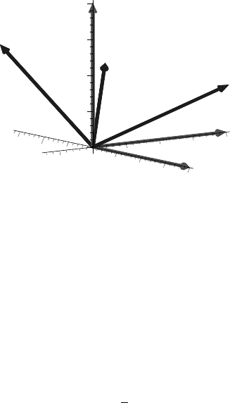
122 CHAPTER 3. VECTORS AND MATRICES
The six arrows are superimposed with the display command with constrained
scaling and a specified orientation of the viewing box, the resulting picture
being shown in Figure 3.7. The original vectors v1 , v2 ,andv3 are the ones
oriented along the coordinate axes.
>
display({seq(a[i],i=1..6)},axes=normal,
orientation=[-36,80],scaling=constrained);
2
4
6
8
–2
4
6
8
–6
–4
2
4
6
8
Figure 3.7: Matrix rotation of three vectors.
3.4 Supplementary Recipes
03-S01: Bobby Blowfly Seeks a Warmer Clime
The temperature in a certain region is given by T =(x−3)
2
+(y−2)
2
+3 (z−1)
2
,
with distances in meters and temperatures in degrees Celsius. Bobby Blowfly
is currently at the point x =1,y =2,z = 3. What is the temperature at this
point? Bobby wishes to start flying in a direction which produces the maximum
rate of temperature increase. What is the unit vector ˆr whichpointsinthis
direction? What is the maximum rate of temperature change at (1, 2, 3)? How
much greater is this rate than if he had decided to fly in the direction given
by the unit vector ˆu =(ˆe
x
− ˆe
y
+ˆe
z
)/
√
3? Plot the 3-dimensional isothermal
(constant temperature) surface passing through the point (1, 2, 3) along with
the unit vectors ˆr and ˆu with their tails placed at the point.
03-S02: Jennifer’s Vector Assignment
Jennifer asks you to try the following problem. Consider the vectors
A =3ˆe
x
− ˆe
y
− 7ˆe
z
,
B =4ˆe
x
+ˆe
y
+2ˆe
z
,and
C =ˆe
x
+5ˆe
y
+4ˆe
z
.
(a) Plot the three vectors as cylindrical arrows in a 3-dimensional picture.
(b) Calculate
P
1
=(
A ×
B) ×
C and
P
2
=
A × (
B ×
C). Confirm
P
1
=
P
2
.
(c) Calculate the volume V = |
A · (
B ×
C)| of a parallelepiped with sides
A,
B,and
C. Show that V =
A
x
A
y
A
z
B
x
B
y
B
z
C
x
C
y
C
z
.
3.4 SUPPLEMENTARY RECIPES 123
03-S03: Another Vector Operator Identity
Using spherical polar coordinates, prove the following vector identity for gen-
eral 3-dimensional vector fields
A and
B:
∇·(
A ×
B)=
B · (∇×
A) −
A · (∇×
B).
03-S04: Another Maple Approach
Using the LinearAlgebra package instead of the VectorCalculus package, derive
the velocity and acceleration of a particle in spherical polar coordinates.
03-S05: Conservative or Non-conservative?
Consider the vector field
A =(3x
2
− 6 yz)ˆe
x
+(2y +3xz)ˆe
y
+(1− 4 xyz
2
)ˆe
z
.
(a) Calculate the line integral of
A along the straight line joining the points
(0, 0, 0) and (1, 1, 1).
(b) Calculate the line integral of
A along the straight lines from (0, 0, 0) to
(0, 0, 1), then to (0, 1, 1), and then to (1, 1, 1).
(c) Calculate the line integral of
A from (0, 0, 0) to (1, 1, 1) along the path
x=t, y =t
2
, z =t
3
,wheret is a parameter.
(d) Having performed the line integrals, is the vector field
A conservative or
non-conservative? Confirm your conclusion by calculating the curl of
A.
(e) Make a 3-dimensional plot of the vector field over an appropriate range of
x, y,andz. Is the distribution of arrows consistent with your conclusion?
03-S06: Basic Matrix Operations
Consider the two square matrices, A =
⎛
⎝
102
2 −13
056
⎞
⎠
,B =
⎛
⎝
2 −11
012
1 −2 −1
⎞
⎠
.
(a) Use the Dimension command to confirm that A and B are 3 × 3 matrices.
(b) By calculating their determinants, show that A and B are non-singular.
(c) Calculate A + B, A − B,andA
2
− B
2
.
(d) Show that AB = BA, i.e., the two matrices do not commute.
(e) Introducing the column vector C =
⎛
⎝
2
1
3
⎞
⎠
, calculate (AB) C.
(f) Show that the product C (AB) is invalid.
(g) Convert C to a row vector C2 by using the Transpose command.
(h) Calculate the product C2(AB).
03-S07: The Cayley–Hamilton Theorem
Given the 4 × 4 matrix
A =
⎛
⎜
⎜
⎝
21−11
−213−2
1 −211
−312−1
⎞
⎟
⎟
⎠
:
124 CHAPTER 3. VECTORS AND MATRICES
(a) Determine the eigenvalues and eigenvectors of A.
(b) Calculate the determinant and trace of A.
(c) Evaluate A
2
, A
3
,andA
4
. Using these results, verify the Cayley–Hamilton
theorem, which states that a matrix satisfies its own characteristic poly-
nomial equation.
03-S08: Simultaneous Diagonalization
Consider the following 4 × 4 matrices,
A =
⎛
⎜
⎜
⎝
1300
3100
0012
0021
⎞
⎟
⎟
⎠
,B=
⎛
⎜
⎜
⎝
2300
3200
0021
0012
⎞
⎟
⎟
⎠
.
(a) Show that AB=BA. The matrices are said to commute.
(b) Determine the eigenvalues of A. Find a general matrix C that reduces A
to diagonal form by the transformation C
−1
AC.
(c) Determine the eigenvalues of B. Show that the matrix C of part (b) also
reduces B to diagonal form by the transformation C
−1
BC.
03-S09: Orthonormal Vectors
Show that the following vectors form an orthonormal set.
A1 =
⎛
⎝
cos(θ)
sin(θ)
0
⎞
⎠
, A2 =
⎛
⎝
−sin(θ)
cos(θ)
0
⎞
⎠
, A3 =
⎛
⎝
0
0
1
⎞
⎠
.
03-S10: Stokes’s Theorem
Stokes’s theorem for a vector field
A states that
C
A · d
=
S
(∇×
A) · da,
where d
is an element of vector path length along the closed contour C and da
is an element of area on the open surface S bounded by C. The direction of the
vector area element is related to the direction of the line integral in a right-hand
sense. Curling the fingers of the right hand in the direction of performing the
line integral, the thumb indicates the sense of the vector area.
Verify Stokes’s theorem for
A=3y ˆe
x
−xzˆe
y
+yz
2
ˆe
z
,whereS is the surface
of the paraboloid 2 z = x
2
+ y
2
bounded by z = 2 and C is its boundary. I.e., C
is the circle x
2
+ y
2
= 4 lying in the x-y plane at z =2.
03-S11: Solving Linear Equation Systems
The currents I
1
, I
2
, I
3
, I
4
in an electrical network satisfy the system of equations
3 I
1
+2I
2
− I
4
=65, 2 I
1
− I
2
+4I
3
+3I
4
= 160,
−7 I
1
− 4 I
2
− 2 I
4
=23, 5 I
1
− I
2
− 2 I
3
+ I
4
=3.
Write the system in matrix form and then determine the currents by (a) using an
inverse matrix approach (b) using the direct approach with the solve command.
Part II
THE ENTREES
The mathematics is not there till we put it there.
Sir Arthur Eddington, The Philosophy of Physical Science, (1882 – 1944)
If scientific reasoning were limited to the logical
processes of arithmetic, we should not get very far
in our understanding of the physical world.
One might as well attempt to grasp the game of poker
entirely by the use of the mathematics of probability.
Vannevar Bush, American scientist (1890 – 1974)
A man ceases to be a beginner in any given science
and becomes a master in that science when he has
learned that...he is going to be a beginner all his life.
R. G. Collingwood, British philosopher (1889–1943)
I believe that a scientist looking at nonscientific
problems is just as dumb as the next guy.
Richard Feynman, American physicist (1918–1988)

Chapter 4
Linear PDEs of Physics
In this chapter, we will solve a wide variety of physical problems involving
linear PDEs, first in Cartesian coordinates, then in other curvilinear coordinate
systems. The common linear PDEs of physics include:
(1) The wave equation (with ψ a continuous scalar function of position r and
time t,andc thewavevelocity),
∇
2
ψ =
1
c
2
∂
2
ψ
∂t
2
, (4.1)
for vibrating elastic strings and membranes, sound waves in fluids, elastic
waves in solids, electromagnetic waves (with ψ a vector), etc.
(2) The diffusion equation (with d a positive diffusion constant),
∂ψ
∂t
= d ∇
2
ψ, (4.2)
which applies to time-dependent heat flow, mixing of fluids, neutron dif-
fusion in nuclear reactors, diffusion of impurities in solids, and so on.
(3) Laplace’s equation,
∇
2
ψ =0, (4.3)
which applies to steady-state heat flow, irrotational flow of an incompress-
ible fluid, and electro(magneto)statics in charge(current)-free regions.
(4) Poisson’s equation (with S asourceterm)
∇
2
ψ = S(r, t), (4.4)
which applies, for example, to the electrostatic potential due to a charge
distribution and to the steady-state temperature with a heat source present.
(5) The time-independent Schr¨odinger equation (with ¯h = h/2π (h being
Planck’s constant), m the mass, V the potential, and E the total energy),
−
¯h
2
2m
∇
2
ψ + Vψ= Eψ, (4.5)
which describes stationary states in quantum mechanics.