Enns R.H. Computer Algebra Recipes for Mathematical Physics

Подождите немного. Документ загружается.

258 CHAPTER 7. CALCULUS OF VARIATIONS

Consider a tiny bug (Betsy Bug) of mass m starting from rest and sliding

under the inﬂuence of gravity along a smooth greased wire from some ﬁxed

point A to another ﬁxed point B somewhere (but not directly) below A.What

should the shape y(x) of the wire be between A and B so that Betsy’s time of

descent is a minimum?

Let’s take the point A to be at the origin (i.e., x

=0, y

= 0) and measure

y downwards. Neglecting friction and air resistance, Betsy’s speed v when she

passes through an arbitrary lower point P (x, y) is obtained by equating her in-

crease in kinetic energy to the decrease in potential energy, i.e.,

= mgy,

or v =

√

2gy,whereg is the acceleration due to gravity. But v = ds/dt where

ds=



(dx)

+(dy)



1+(y



)

dx is an element of arc length along the path

at P and dt is the time it takes for Betsy to traverse ds. Combining these

results, the time T of descent from A to B(where x = x

,y = y

)is

T =





1+(y



)

√

2gy

The y(x) which minimizes T follows on solving (7.2) with F =



1+(y



)

√

2gy.

In this recipe, we will derive Betsy’s path in the parametric form

x =

(θ −sin θ),y=

(1 − cos θ),

with θ a parameter which is equal to 0 at A. Then, taking θ= θ1 at B, we will

show that the minimum time of descent is T =



a/2gθ1 . Finally, choosing

=5m,y

= 2 m, Betsy’s path will be plotted and T evaluated.

If the form of F is speciﬁed, the EulerLagrange command will calculate the

left-hand side of (7.2), and even produce the ﬁrst integral if possible. To use

this command, the VariationalCalculus package must be ﬁrst loaded.

restart: with(VariationalCalculus):

The relevant F for the brachistochrone problem is entered. The factor 1/

√

is omitted since it will cancel out of the Euler–Lagrange equation, (7.2).

F:=sqrt(1+diff(y(x),x)ˆ2)/sqrt(y(x));

F :=



1+(

y(x))



y(x)

The EulerLagrange command, with F , x,andy(x) given as arguments, is

applied to F and simpliﬁed, generating two results.

eq:=simplify(EulerLagrange(F,x,y(x)));

eq :=

⎧

⎪

⎨

⎪

⎩



1+(

y(x))



y(x)

= K

, −

1+(

y(x))

+2(

y(x)) y(x)

y(x)

(3/2)

(1+(

y(x))

)

(3/2)

⎫

⎪

⎬

⎪

⎭

Since F doesn’t explicitly depend on x here, the ﬁrst integral is generated in

the ﬁrst expression in the above output, the integration constant being K

The second expression is just the left-hand side of the resulting ODE generated

7.1. EULER–LAGRANGE EQUATION 259

by the Euler–Lagrange equation. We will work with the ﬁrst integral and now

select it in eq2 . The last argument, [1], in the command line removes the curly

(Maple set) brackets which would otherwise enclose the ﬁrst integral expression.

eq2:=select(has,eq,K[1])[1];

eq2 :=



1+(

y(x))



y(x)

= K

The dsolve command is used to analytically solve eq2 for y(x). The parametric

option is speciﬁed, since a parametric form of the solution is desired.

sol:=dsolve(eq2,y(x),parametric);

sol :=

T )=

(1 + T

)

T )=

−

T − arctan( T ) − arctan( T ) T

+ C1 K

(1 + T

)

The mathematical forms of x and y are given in terms of the parameter

T .The

quantity

C1 is a second integration constant. A new parameter θ is introduced

by setting

T = cos(θ/2)/ sin(θ/2). The constant K

is set equal to 1/

√

_T:=cos(theta/2)/sin(theta/2): K[1]:=1/sqrt(a):

Let’s tackle x ﬁrst. The right-hand side of the second expression in sol is

symbolically simpliﬁed with the trig option, the above assignments having been

automatically substituted.

x:=simplify(rhs(sol[2]),trig,symbolic);

x := −cos(

) a sin(

) − arctan

⎛

⎜

⎝

cos(

)

sin(

)

⎞

⎟

⎠

a +

Applying the combine command with the trig option reduces the ﬁrst term in

x to one of the terms desired in the ﬁnal form of x.

x:=combine(x,trig);

x := −

a sin(θ) − arctan

⎛

⎜

⎝

cos(

)

sin(

)

⎞

⎟

⎠

a +

We must choose the constant

C1 in such a way that the last two terms in the

above output reduce to aθ/2. To do this, recall that the parameter θ must have

the value 0 when x=0. For θ=0, the ﬁrst term in the above output is 0, while

the second term yields −a arctan(∞), or −aπ/2. Thus, to make θ =0 at x=0,

we must choose

C1 = aπ/2. This substitution is now made in x. We further

substitute cos(θ/2)= cot(θ/2) sin(θ/2).

x:=subs({_C1=a*Pi/2,cos(theta/2)=cot(theta/2)*sin(theta/2)},x );

260 CHAPTER 7. CALCULUS OF VARIATIONS

x := −

a sin(θ) − arctan(cot(

)) a +

aπ

Applying the combine command with the trig option, and then making the

substitution arccot(cot(θ/2))= θ/2 produces the desired ﬁnal form for x.

x:=combine(x,trig);

x := −

a sin(θ)+a arccot(cot(

))

x:=subs(arccot(cot(theta/2))=theta/2,x);

x := −

a sin(θ)+

aθ

Next, we tackle y by selecting the ﬁrst expression from the right-hand side of

sol and simplifying with the trig and symbolic options.

y:=simplify(rhs(sol[1]),trig,symbolic);

y := a sin(

)

Applying combine, with the trig option, yields the ﬁnal desired form of y.

y:=combine(y,trig);

y :=

−

a cos(θ)

With the parametric forms of x and y determined, the minimum time of descent

can be calculated. First note that the time of descent

T =







dy(x)





2 gy(x)



θ1





dy(θ)/dθ

dx(θ)/dθ





dx(θ)

dθ



dθ



2 gy(θ)

where θ1 is the value of θ at the end point B. The latter integrand is now

calculated and simpliﬁed assuming that θ>0.

integrand:=simplify(sqrt(1+(diff(y,theta)/diff(x,theta))ˆ2)

*diff(x,theta)/sqrt(2*g*y)) assuming theta>0;

integrand :=

√

2 a

√

The minimum time of descent, assigned the name T , follows on integrating the

integrand from θ =0 to θ1 .

T:=int(integrand,theta=0..theta1);

T :=

√

2 aθ1

√

The value of θ1 depends on the coordinates x

, y

of the point B, and must be

determined numerically. This is now done for the speciﬁed values x

=5, y

=2.

x1:=x=5; y1:=y=2;

x1 := −

a sin(θ)+

aθ

=5 y1 :=

−

a cos(θ)=2

7.1. EULER–LAGRANGE EQUATION 261

The above pair of equations is solved numerically for the constant a and the

value of θ at B, i.e., θ1 .

sol2:=fsolve({x1,y1},{a,theta});

sol2 := {θ =3.819665136,a=2.248728127}

Thevaluesofθ1 and a are now expressed separately.

theta1:=eval(theta,sol2); a:=eval(a,sol2);

θ1 := 3.819665136 a := 2.248728127

Betsy’s path then is given by the following expressions for x and y. Taking

g =9.8m/s

, her time of descent is also calculated.

x:=x; y:=y; g:=9.8: T:=evalf(T);

x := −1.124364064 sin(θ)+1.124364064 θ

y := 1.124364064 −1.124364064 cos(θ)

T := 1.293795782

Along the path given by the above forms of x and y, Betsy takes about 1.29

seconds to travel from the origin (A)toB. This is the minimum time possible

between these points, any other path producing a longer time. If you don’t

believe it, try calculating the time for descent along, e.g., a straight line path

between A and B.

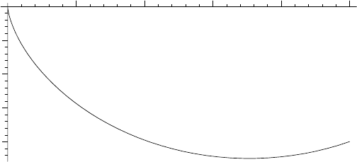
Finally, Betsy’s path is plotted from θ =0 to θ1 with constrained scaling.

The resulting picture is shown in Figure 7.1. Mathematically, the path is a

portionofaninvertedcycloid. Another example of a cycloidal path is the

trajectory traced out by a point on the rim of a wheel rolling without slipping.

plot([x,-y,theta=0..theta1],scaling=constrained,

thickness=2,labels=["x","y"]);

–2

–1

12345

Figure 7.1: Betsy’s path which minimizes the time of descent.

262 CHAPTER 7. CALCULUS OF VARIATIONS

7.1.2 Fermat’s Principle

The light that radiates from the great novels time can never dim....

Milan Kundera, Czech author, critic, (1929–)

Fermat’s principle states that a ray of light in a medium with a variable re-

fractive index n will follow the path which requires the shortest traveling time.

Consider a medium which has a refractive index n(x, y)=e

,withx the hori-

zontal and y the vertical coordinate, respectively. Noting that the speed of light

is v = c/n,wherec is the vacuum speed of light, determine the general equation

for the light ray path. Taking a = 1, determine the light ray path between the

points (−1, 1) and (1, 1) and plot it.

Now the light ray speed v = ds/dt = c/n,whereds =



(dx)

+(dy)



1+(y



)

dx is an element of arclength and dt is a time interval. So, since

n= e

, the total time to travel between x=−1 and +1 is given by

T =



−1



1+(y



)

dx.

Omitting the constant factor 1/c which cancels out, the Euler–Lagrange equa-

tion will be solved with F =e



1+(y



)

. As in the previous recipe, since F

doesn’t explicitly depend on x, a ﬁrst integral must exist.

After loading the VariationalCalculus package, the refractive index n is en-

tered and F formed.

restart: with(VariationalCalculus):

n:=exp(a*y(x)); F:=n*sqrt(1+diff(y(x),x)ˆ2);

n := e

(a y(x))

F := e

(a y(x))



1+(

y(x))

The EulerLagrange command is applied to F and the result simpliﬁed.

eq:=simplify(EulerLagrange(F,x,y(x)));

eq :=

⎧

⎪

⎨

⎪

⎩

(a y(x))



1+(

y(x))

= K

, −

(a y(x))

(−a − a (

y(x))

y(x)))

(1+(

y(x))

)

(3/2)

⎫

⎪

⎬

⎪

⎭

In addition to generating the left-hand side of the Euler–Lagrange equation (sec-

ond term in eq ), the ﬁrst integral has been generated (ﬁrst term) as expected.

Once again, we will work with the ﬁrst integral, selecting the expression from

eq which contains the constant K

eq2:=select(has,eq,K[1])[1];

eq2 :=

(a y(x))



1+(

y(x))

= K

7.1. EULER–LAGRANGE EQUATION 263

Then, eq2 is analytically solved for y(x) using the dsolve command and as-

suming that K

is real. If this assumption is not made, a much more formidable

form of the solution will occur. Further, even with the assumption included,

there occasionally may appear more possible forms of y(x) in the output of sol.

If this occurs, either select the solution which corresponds to the one chosen

here or re-execute the work sheet to get an identical output.

sol:=dsolve(eq2,y(x)) assuming K[1]::real;

sol := y(x)=

ln(K

)

, y(x)=

ln(



tan(a (x − C1 ))

+1K

tan(a (x − C1 ))

)

y(x)=

ln(−



tan(a (x − C1 ))

+1K

tan(a (x − C1 ))

)

Noting that the second and third solutions in sol turn out to be equivalent, the

rhs of the third solution is chosen and converted to sines and cosines.

y:=convert(rhs(sol[3]),sincos);

y :=

⎛

⎜

⎝

−



sin(a (x −

C1 ))

cos(a (x −

C1 ))

+1K

cos(a (x − C1 ))

sin(a (x − C1 ))

⎞

⎟

⎠

The form of y is considerably simpliﬁed in y2 by applying the radical simpliﬁ-

cation command followed by combine with the trig option.

y2:=combine(radsimp(y),trig);

y2 :=

ln(−

sin(ax− a

C1 )

)

With an analytic form for the light ray path determined, the given parameter

values are now entered. Here h is the vertical coordinate of the end points of

the light ray path and x=±L will be the end points’ horizontal coordinates.

a:=1: h:=1: L:=1:

The light ray must pass through the points (x= L, y = h)and(−L, h). These

boundary conditions are entered in bc1 and bc2 , respectively.

bc1:=eval(y2,x=L)=h; bc2:=eval(y2,x=-L)=h;

bc1 := ln(

sin(−1+

C1 )

)=1 bc2 := ln(

sin(1 +

C1 )

)=1

Then bc1 and bc2 are numerically solved for K

and C1 and the solution

assigned. K

and C1 are automatically substituted into y2 which is displayed.

sol2:=fsolve({bc1,bc2},{K[1],_C1}); assign(sol2): y2:=y2;

sol2 := {

C1 = −7.853981634,K

= −1.468693940}

264 CHAPTER 7. CALCULUS OF VARIATIONS

y2 := ln(

1.468693940

sin(x +7.853981634)

)

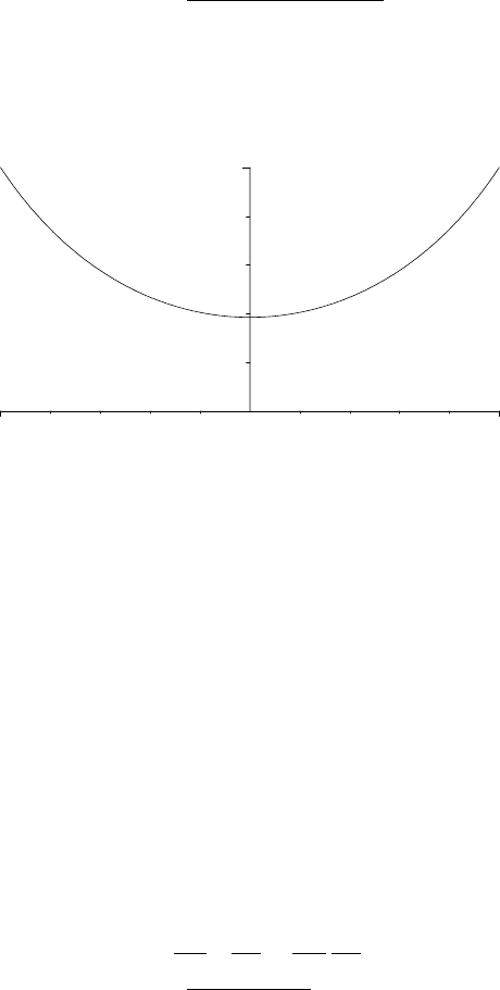
The solution y2 is now plotted with constrained scaling,

plot(y2,x=-L..L,thickness=2,tickmarks=[3,2],view=

[-L..L,0..h],scaling=constrained,labels=["x","y"]);

–1 1

Figure 7.2: Path traced by light ray between the points (−1, 1) and (1, 1).

the light ray path being shown in Figure 7.2. The path joining the two points

is curved rather than a straight line.

7.1.3 Betsy’s Other Path

Adulthood is the ever-shrinking period between childhood and old age.

It is the apparent aim of modern industrial societies to reduce this

period to a minimum.

Thomas Szasz, American psychiatrist, The Second Sin,“Social Relations” (1973)

Suppose that we want to ﬁnd the function y(x) which minimizes or maximizes

I[y]=



F (x, y, y



) dx,withy ﬁxed at x

, but with the other end point x

free to lie anywhere along the curve G(x, y) = 0. According to Mathews and

Walker [MW71], y(x) may still be found by solving the Euler–Lagrange equa-

tion, but subject to the subsidiary condition



F −y



∂F

∂y





∂G

∂y

−

∂F

∂y



∂G

∂x

=0. (7.4)

For the brachistochrone, F =



(1 + (y



)

)/y and the condition (7.4) reduces

to y



=(∂G/∂y)/(∂G/∂x). I.e., the curve of quickest descent must intersect

G(x, y) =0 at right angles.

As a simple illustration of applying this latter condition, suppose that Betsy

bug now slides down a smooth wire from the origin (starting at rest, and with y

measured downwards) to the parabola y =mx

+ c, where the parabola passes

7.1. EULER–LAGRANGE EQUATION 265

through the two points (x=0,y =50) and (30, 0) cm. Determine the path which

minimizes Betsy’s time of descent to the parabola. Taking g =980 cm/s

,how

long does it take Betsy to reach the parabola and through what distance does

she drop? Plot Betsy’s path and the parabola, using constrained scaling.

After loading the plots package, the parabolic equation G is entered.

restart: with(plots):

G:=Y-m*Xˆ2-c=0;

G := Y − mX

− c =0

Evaluating G at the two given points and solving yields the values of m and c.

sol:=solve({eval(G,{X=0,Y=50}),eval(G,{X=30,Y=0})},{m,c});

sol := {c =50,m=

−1

}

Assigning sol, the explicit form of the parabola G then is as follows.

assign(sol): G:=G;

G := Y +

− 50 = 0

The quantity (∂G/∂Y )/(∂G/∂X) is calculated and evaluated at the (still un-

known) end point X =x

s:=eval(lhs(diff(G,Y))/lhs(diff(G,X)),X=x1);

s :=

Since F isthesameasinRecipe07-1-1, the path of quickest descent must

have the same mathematical form as obtained earlier. In parametric form, the

equations describing the x and y coordinates of the path are as follows:

x:=(a/2)*(theta-sin(theta)); y:=(a/2)*(1-cos(theta));

x :=

a (θ − sin(θ)) y :=

a (1 − cos(θ))

The slope of the path, dy/dx or (dy/dθ)/(dx/dθ), must be equal to s at some

unknown value θ1 of the parameter θ. This boundary condition is now entered.

bc||1:=eval(diff(y,theta)/diff(x,theta),theta=theta1)=s;

bc1 :=

sin(θ1)

1 − cos(θ1)

As two additional conditions, x and y evaluated at θ = θ1 must be equal to x1

and y1 . Finally, in bc4 we evaluate G at X = x1 and Y = y1 .

bc||2:=x1=eval(x,theta=theta1);

bc2 := x1 =

a (θ1 − sin(θ1))

bc||3:=y1=eval(y,theta=theta1);

bc3 := y1 =

a (1 − cos(θ1))

bc||4:=eval(G,{X=x1,Y=y1});

266 CHAPTER 7. CALCULUS OF VARIATIONS

bc4 := y1 +

− 50 = 0

The 4 boundary conditions are numerically solved for x1 , y1 , a,andθ1.

sol2:=fsolve({seq(bc||i,i=1..4)},{x1,y1,a,theta1},x1=0..30);

sol2:={a =26.49236117,x1 =22.15176281,θ1= 2.369761726,y1 =22.73885580}

Assigning sol2 , the parametric equations describing Betsy’s path are as follows:

assign(sol2): x:=x; y:=y;

x := 13.24618058 θ −13.24618058 sin(θ)

y := 13.24618058 −13.24618058 cos(θ)

Entering the value of g, the distance h through which Betsy drops and the

(minimum) time T it takes to reach the parabola are calculated. h is given by

the numerical value of y1, while for T we borrow the result T =



a/(2g) θ from

recipe 07-1-1 and evaluate it at θ = θ1.

g:=980: h:=evalf(y1); T:=evalf(sqrt(a/(2*g))*theta1);

h := 22.73885580 T := 0.2755097538

Betsy drops through 22.7 cm and takes about 0.28 seconds to reach the parabola.

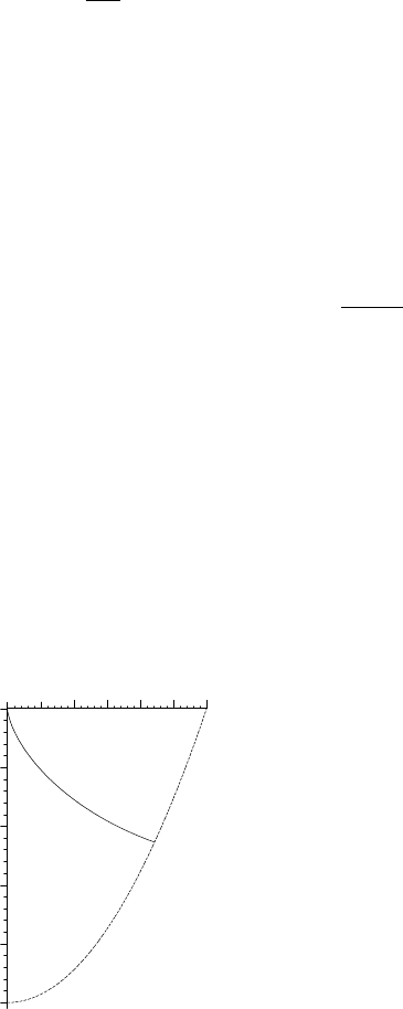
In gr1 and gr2, Betsy’s path and the parabola are plotted, respectively.

gr1:=plot([x,-y,theta=0..theta1],color=blue,thickness=2):

gr2:=plot(lhs(G)-Y,X=0..30,thickness=2,linestyle=3):

The two graphs are superimposed with the display command, constrained

scaling being used. The resulting picture is shown in Figure 7.3, the solid curve

being Betsy’s path, the dashed curve the parabola.

display({gr1,gr2},scaling=constrained,labels=["x","y"]);

–50

15 30

Figure 7.3: Betsy’s path which minimizes the time of descent to the parabola.

Since constrained scaling has been used, it may be seen from the ﬁgure that

Betsy’s path does indeed intersect the parabola at right angles.

7.2. SUBSIDIARY CONDITIONS 267

7.2 Subsidiary Conditions

In diﬀerential calculus, we may require a function φ(x, y)tobeaconditional

minimum or maximum subject to a subsidiary condition y = y

(x)or,equiva-

lently g(x, y)= 0. How is a conditional extremum calculated?

A straightforward way is to replace y in φ(x, y)withy

(x) and calculate

dφ(x, y

(x))

=0, or using the chain rule,

∂φ

∂x

∂φ

∂y

∂x

=0. (7.5)

An alternate procedure is the method of Lagrange multipliers. One extrem-

izes φ + λg, subject to g(x, y)=0. λ is called the Lagrange multiplier. More

explicitly, one must solve the simultaneous equations

∂

∂x

(φ + λg)=0,

∂

∂y

(φ + λg)=0,g=0. (7.6)

In variational calculus, we may require an integral I[y]=



F (x, y, y



) dx

to be a minimum or maximum subject to an integral subsidiary condition

N =



G(x, y, y



)=C,whereC is a known constant. In this case, one sets

F=F + λG and solves the Euler–Lagrange equation

∂F

∂y

−



∂F

∂y





=0. (7.7)

Extensions can be made to handle more than one subsidiary condition. In the

following recipes, examples from diﬀerential and variational calculus are given.

7.2.1 Ground State Energy

Authority has always attracted the lowest elements in the human

race. All through history mankind has been bullied by scum...Every

government is a parliament of whores. The trouble is, in a democ-

racy the whores are us.

P. J. ORourke, American journalist, (1947–)

The quantum mechanical ground state energy of a particle of mass m in a

box (rectangular parallelepiped) with sides a, b, c, is given ([Wie73]) by

E =

¯h

2 m





where ¯h = h/(2π), h being Planck’s constant.

What shape must the box have to minimize the energy E, subject to the

constraint that the volume V = abc of the box is constant? What is the

minimum energy? Solve this problem by (a) the “direct” method, (b) the

method of Lagrange multipliers. Here is Ms. I. M. Curious’s solution.

(a) I. M. enters the energy expression E, setting A ≡ (¯h

)/(2 m).

restart: E:=A*(1/aˆ2+1/bˆ2+1/cˆ2);

E := A (

)