Enns R.H. Computer Algebra Recipes for Mathematical Physics

Подождите немного. Документ загружается.

268 CHAPTER 7. CALCULUS OF VARIATIONS

The volume V = abc is constant, so I. M. eliminates the variable c by setting

c= V/(ab). The new form of E is then displayed.

c:=V/(a*b): E:=E;

E := A (

)

To determine the values of a and b which will extremize E, she sets ∂E/∂a =0

and ∂E/∂b=0 in eq1 and eq2 , respectively.

eq1:=diff(E,a)=0; eq2:=diff(E,b)=0;

eq1 := A (−

2 ab

)=0 eq2 := A (−

2 a

)=0

For the extremum to be a minimum, I. M. notes that one must have [Ste87]

∂

∂a

> 0, and



∂

∂a



∂

∂b



−



∂

∂a∂b



> 0.

The left-hand sides of these two conditions are now entered in eq3a and eq3b.

eq3a:=diff(E,a,a);

eq3b:=diff(E,a,a)*diff(E,b,b)-diff(E,a,b)ˆ 2;

eq3a := A (

2 b

) eq3b := A

(

2 b

)(

2 a

) −

16 A

Clearly ∂

E/∂a

is positive, but it is not yet clear whether the second expression

in the above output is also positive. I. M. now solves eq1 and eq2 for a and b.

sol:=solve({eq1,eq2},{a,b});

sol := {a = RootOf(−V +

),b= RootOf(−V + Z

)}, ....

Four possible solutions for a and b are generated in sol, all expressed as RootOf.

These four solutions are now converted to radical forms in sol2 .

sol2:=seq(convert(sol[i],radical),i=1..4);

sol2 := {a = V

(1/3)

,b= V

(1/3)

}, {a = −(−V )

(1/3)

,b=(−V )

(1/3)

{a = −V

(1/3)

,b= V

(1/3)

}, {a =(−V )

(1/3)

,b=(−V )

(1/3)

}

Clearly, the ﬁrst solution in sol2 is the desired one, which I. M. now assigns.

Thevaluesofa, b, c, and the minimum energy, Emin, immediately follow.

assign(sol2[1]): a:=a; b:=b; c:=c; Emin:=E;

a := V

(1/3)

b := V

(1/3)

c := V

(1/3)

Emin :=

3 A

(2/3)

To minimize the energy, the box must be cubical. That the energy is a minimum

follows on displaying eq3a and eq3b, which are both positive.

eq3a:=eq3a; eq3b:=eq3b;

eq3a :=

8 A

(4/3)

eq3b :=

48 A

(8/3)

(b) Now, I. M. uses the method of Lagrange multipliers. The energy expression

E is entered along with g ≡ abc − V. The subsidiary condition is g =0.

7.2. SUBSIDIARY CONDITIONS 269

restart: E:=A*(1/aˆ2+1/bˆ2+1/cˆ2); g:=a*b*c-V;

E := A (

) g := abc− V

I. M. forms a functional operator f to diﬀerentiate E + λg with respect to an

arbitrary variable v, and then set the result equal to zero.

f:=v->diff(E+lambda*g,v)=0:

Then f is used, with v equal to a, b,andc in eq1 , eq2 ,andeq3 , respectively.

The relation g = 0 is given in eq4 .

eq||1:=f(a); eq||2:=f(b); eq||3:=f(c); eq||4:=g=0;

eq1 := −

2 A

+ λbc=0 eq2 := −

2 A

+ λac=0

eq3 := −

2 A

+ λab=0 eq4 := abc− V =0

The sequence of four equations is solved for a, b, c,andλ, and each of the

solutions converted from RootOf forms to radical notation.

sol:=solve({seq(eq||i,i=1..4)},{a,b,c,lambda}):

sol2:=seq(convert(sol[i],radical),i=1..4);

sol2 := {b = V

(1/3)

,c= V

(1/3)

,a= V

(1/3)

,λ=

2 A

(5/3)

}, ....

The ﬁrst solution in sol2 is assigned and a, b, c,andEmin displayed.

assign(sol2[1]): a:=a; b:=b; c:=c; Emin:=E;

a := V

(1/3)

b := V

(1/3)

c := V

(1/3)

Emin :=

3 A

(2/3)

As I. M. expected, the answer agrees with that obtained with the direct method.

7.2.2 Erehwon Hydro Line

The fundamental concept in social science is Power, in the same

sense in which Energy is the fundamental concept in physics.

Bertrand Russell, British philosopher, mathematician, (1872–1970)

Erehwon Hydro has suspended a power line, of length L =1.5 km and lin-

ear mass density  = 1000 kg/km, across a deep, wide, gorge. Relative to the

origin at the gorge bottom, the two towers from which the cable is suspended

are at (−a/2,b)and(a/2,b), where a =1.25 km and b = 1 km. Assuming

that the equilibrium shape of the cable is such as to minimize the potential en-

ergy, determine the cable shape and plot it. Take the gravitational acceleration

g =9.8/1000 km/s

. What is the distance between the lowest point in the cable

and the gorge bottom?

If an arclength element ds=



1+(y



)

dx of cable at a point x is a distance

y(x) above the gorge bottom, the potential energy of the whole cable is

270 CHAPTER 7. CALCULUS OF VARIATIONS

V =



dsgy=



a/2

−a/2

gy



1+(y



)

dx.

After loading the VariationalCalculus package,

restart: with(VariationalCalculus):

the integrand F = gy



1+(y



)

of the potential energy V is entered.

F:=epsilon*g*y(x)*sqrt(1+diff(y(x),x)ˆ2);

F := εgy(x)



1+(

y(x))

The subsidiary condition is that the length of the cable must be L, i.e.,



ds =



a/2

−a/2



1+(y



)

dx = L.

The integrand G=



1+(y



)

of this constraint relation is entered,

G:=sqrt(1+diff(y(x),x)ˆ2);

G :=



1+(

y(x))

and the combination FF =F + λG formed, where λ is the Lagrange multiplier.

FF:=simplify(F+lambda*G);

FF :=



1+(

y(x))

(εgy(x)+λ)

The EulerLagrange command is applied to FF and simpliﬁed. Since FF

doesn’t explicitly depend on x, in addition to the lhs of the Euler–Lagrange

equation, a ﬁrst integral is generated, the integration constant being K

eq:=simplify(EulerLagrange(FF,x,y(x)));

eq :=

⎧

⎪

⎨

⎪

⎩

εgy(x)+λ



1+(

y(x))

= K

εg+ εg(

y(x))

− (

y(x)) εgy(x) − (

y(x)) λ

(1 + (

y(x))

)

(3/2)

⎫

⎪

⎬

⎪

⎭

The select command is used to extract the ﬁrst integral relation.

eq2:=select(has,eq,K[1])[1];

eq2 :=

εgy(x)+λ



1+(

y(x))

= K

The ODE in eq2 is analytically solved for y(x), assuming that >0, g>0.

sol:=dsolve(eq2,y(x)) assuming epsilon>0,g>0;

7.2. SUBSIDIARY CONDITIONS 271

Two equivalent solutions (not shown here) are produced in sol , the rhs of the

second solution being chosen, simpliﬁed, and assigned the name Y .

Y:=simplify(rhs(sol[2]));

Y :=

+ e

(−

2 εg(x− C1 )

)

− 2 e

(−

εg(x− C1 )

)

λ) e

(

εg(x− C1 )

)

εg

The solution Y is converted to a trig form, and the combine command applied.

Y2:=combine(convert(Y,trig));

Y2 :=

cosh(

εg(x −

C1 )

)+K

sinh(

εg(x −

C1 )

)

+cosh(

εg(x −

C1 )

) − sinh(

εg(x −

C1 )

) − 2 λ)



(εg)

The cosh and sinh terms are collected in Y2 .

Y3:=collect(Y2,[cosh,sinh]);

Y3 :=

(1+K

)cosh(

εg(x − C1 )

)

εg

− 1) sinh(

εg(x − C1 )

)

εg

−

εg

To evaluate the constants K

C1, and λ, three conditions are needed. Since

the cable will hang symmetrically, the slope at the center of the cable (x =0)

must be zero. This is entered as boundary condition bc1 .Attheendpoint

x=a/2, the vertical coordinate is b.Thisisenteredinbc2 .

bc1:=eval(diff(Y3,x),x=0)=0: bc2:=eval(Y3,x=a/2)=b:

The two boundary conditions are solved for λ and

C1.

sol2:=solve({bc1,bc2},{lambda,_C1}): assign(sol2):

After assigning sol2 , the cable shape is given by Y4 .

Y4:=expand(Y3);

Y4 :=

cosh(

εgx

) K

εg

−

cosh(

aεg

) K

εg

+ b

The constant K

remainstobeevaluated. Theconstraint



a/2

−a/2

Gdx= L is

applied in bc3 . To perform the integration, it is assumed that a>0, >0,

g>0, and K

> 0.

bc3:=simplify(int(eval(G,y(x)=Y4),x=-a/2..a/2))=L

assuming a>0,epsilon>0,g>0,K[1]>0;

bc3 :=

(−1/2

aεg

)

(−1+e

(

aεg

)

εg

= L

bc3 is a transcendental equation, which must be solved numerically for K

.The

given parameter values are entered.

epsilon:=1000: L:=1.5: a:=1.25: b:=1: g:=9.8/1000:

272 CHAPTER 7. CALCULUS OF VARIATIONS

Then bc3 is numerically solved for K

, the value being labeled K1. Evaluating

Y4 at K

=K1 , the equilibrium shape of the cable is given by Y5 .

K1:=fsolve(bc3,K[1]=0..10); Y5:=eval(Y4,K[1]=K1);

K1 := 5.751883654

Y5 := 0.5869269033 cosh(1.703789678 x)+0.0476433492

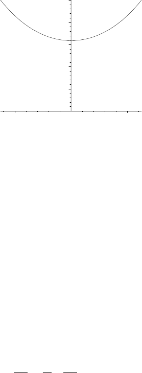
The equilibrium shape Y5 , called a catenary, is plotted with constrained scal-

ing, the resulting picture being shown in Figure 7.4.

plot(Y5,x=-a/2..a/2,thickness=2,view=[-a/2..a/2,0..b],

scaling=constrained,tickmarks=[3,3],labels=["x","y"]);

0.2

0.4

0.6

0.8

–0.5 0.5

Figure 7.4: Equilibrium shape of the power line.

Evaluating Y5 at x =0, the lowest point on the cable

height:=eval(Y5,x=0);

height := 0.6345702525

is about 0.635 km, or 635 m, above the gorge bottom.

7.3 Lagrange’s Equations

In classical mechanics, the Lagrangian L is deﬁned by L = T − V ,whereT

is the kinetic energy and V the potential energy of the system of interest. If

L= L(q

, ˙q

,t)whereq

are the generalized coordinates (any set of coordinates

completely specifying the state of the system), ˙q

the (generalized) velocity com-

ponents, and t the time, then Hamilton’s principle states that of all possible

motions the actual motion of the system over a time interval t

to t

is the one

for which



L(q

, ˙q

,t) dt is an extremum. Setting the variation of the integral

equal to zero leads to Lagrange’s equations of motion

∂L

∂q

−



∂L

∂ ˙q



=0, (7.8)

which are equivalent to Newton’s law of motion. Since (7.8) is of the same

structure as Eq. (7.2), we can also make use of the EulerLagrange command.

7.3. LAGRANGE’S EQUATIONS 273

7.3.1 Daniel’s Chaotic Pendulum

Out of chaos God made a world,

and out of high passions comes a people.

Lord Byron, English poet, (1788–1824)

Daniel’s engineering father has given him a toy for his birthday which basi-

cally consists of a simple pendulum (a small mass m attached to the end of a

lightrodoflengthb), whose pivot point is attached to the rim of a wheel of

radius a which rotates at a constant angular velocity ω. The pendulum is in

the same vertical plane as the wheel and is free to rotate completely about its

pivot point. All frictional eﬀects are neglected. This recipe will determine the

equation of motion for m, numerically solve the resulting nonlinear ODE, and

animate the motion. The plots and VariationalCalculus packages are loaded.

restart: with(plots): with(VariationalCalculus):

If θ(t) is the angle that the pendulum rod makes with the vertical, the horizontal

coordinate of m at time t is x= a cos(ωt)+b sin(θ(t)) which is entered.

x:=a*cos(omega*t)+b*sin(theta(t));

x := a cos(ωt)+b sin(θ(t))

The vertical coordinate of m at time t is y =a sin(ωt) − b cos(θ(t)).

y:=a*sin(omega*t)-b*cos(theta(t));

y := a sin(ωt) − b cos(θ(t))

The horizontal ( ˙x)andvertical(˙y) components of m’s velocity are calculated.

xdot:=diff(x,t); ydot:=diff(y,t);

xdot := −a sin(ωt) ω + b cos(θ(t)) (

θ(t))

ydot := a cos(ωt) ω + b sin(θ(t)) (

θ(t))

The kinetic (T =

m (˙x

+˙y

)) and potential (V = mgy) energy are determined.

T:=simplify(m*(xdotˆ2+ydotˆ2)/2); V:=m*g*y;

T :=

m(a

− 2 a sin(ωt) ωbcos(θ(t)) (

θ(t))

+2a cos(ωt) ωbsin(θ(t)) (

θ(t)) + b

(

θ(t))

)

V := mg(a sin(ωt) −b cos(θ(t)))

The Lagrangian L=T −V is formed, T being simpliﬁed by applying the combine

command with the trig option.

L:=combine(T,trig)-V;

L :=

− maωb(

θ(t)) sin(ωt− θ(t)) +

(

θ(t))

− mg(a sin(ωt) − b cos(θ(t)))

274 CHAPTER 7. CALCULUS OF VARIATIONS

The governing equation of motion, ode , is obtained by applying the

EulerLagrange command as follows. Because L depends explicitly on t,a

ﬁrst integral is not generated with the EulerLagrange command.

ode:=simplify(-EulerLagrange(L,t,theta(t))[1]/(m*b))=0;

ode := g sin(θ(t)) − aω

cos(ωt− θ(t)) + b (

θ(t)) = 0

Since ode is a nonlinear ODE, it must be solved numerically. We will consider

a giant version of Daniel’s toy taking a=1 m and b=3 m. The wheel is rotated

at ω =2 rads/s and g =9.8m/s

. The ODE is then displayed in ode2 .

a:=1: b:=3: omega:=2: g:=9.8: ode2:=ode;

ode2 := 9.8sin(θ(t)) − 4 cos(2 t − θ(t)) + 3 (

θ(t)) = 0

For the initial condition, let’s take θ(0)= π/6radsand

θ(0)= 0.

ic:=theta(0)=Pi/6,D(theta)(0)=0:

Then, ode2 is numerically solved in sol, subject to the initial condition, for

θ(t). The output is given as a listprocedure.

sol:=dsolve({ode2,ic},theta(t),type=numeric,

output=listprocedure):

Making use of sol, the next three command lines allow us to evaluate the

horizontal and vertical coordinates of m at an arbitrary time t.

Theta:=eval(theta(t),sol):

X:=t->eval(x,theta(t)=Theta(t)):

Y:=t->eval(y,theta(t)=Theta(t)):

The circle command, found in the plottools library package, is used to plot a

thick red circle of radius a, centered on the origin, representing the wheel’s rim.

c:=plottools[circle]([0,0],a,color=red,style=line,

thickness=2):

The line command (also in the plottools package) is used to create an arrow

operator l to draw the pendulum rod as a thick green line at arbitrary time t.

l:=t->plottools[line]([a*cos(omega*t),a*sin(omega*t)],

[X(t),Y(t)],color=green,thickness=2):

The pointplot command is used to form an operator p to draw size 16 blue

circles at the pivot point and at m at arbitrary time t.

p:=t->pointplot({[a*cos(omega*t),a*sin(omega*t)],

[X(t),Y(t)]},symbol=circle,symbolsize=16,color=blue):

The three graphs are superimposed in gr||i at a time t =0.1 i,andadoloop

used to generate plots for i from 0 to 200, i.e, for t=0 to 20 s.

for i from 0 to 200 do

t:=0.1*i:

gr||i:=display({c,p(t),l(t)},labels=["x","y"]):

end do:

7.3. LAGRANGE’S EQUATIONS 275

The motion of the pendulum is animated by displaying the sequence of graphs,

using the insequence=true option.

display(seq(gr||i,i=0..200),insequence=true);

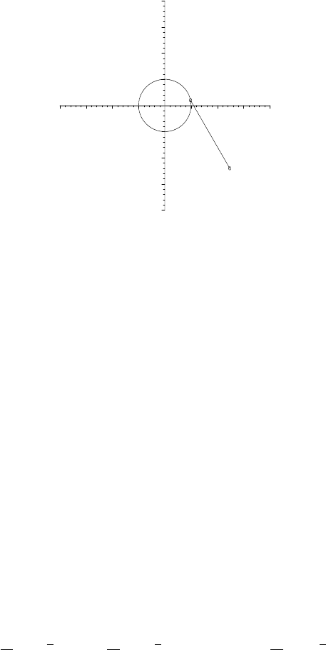
A typical (at t=0.1 s) frame of the animation is shown in Figure 7.5. Click on

the computer plot and on the start arrow to see the entire pendulum motion.

–4

–4 4

Figure 7.5: Typical frame of the animation of Daniel’s chaotic pendulum.

For the choice of parameter values, the motion is quite irregular or “chaotic”

in appearance. You should try other values and see what happens.

7.3.2 Van Allen Belts

He could not see a belt without hitting below it.

Margot Asquith, British socialite about a former prime minister, (1864–1945)

As an interesting and non-trivial example, in this recipe we will determine

and animate the motion of a proton moving in the magnetic dipole ﬁeld of the

earth. The animated motion is characteristic of the behavior of charged parti-

cles trapped in the Van Allen radiation belts surrounding the earth. [Bra68]

This recipe uses the plots, VariationalCalculus, and VectorCalculus pack-

ages which will generate several warnings unless suppressed, e.g., by using the

interface command to set the warnlevel to 0.

restart: interface(warnlevel=0):

with(plots): with(VariationalCalculus): with(VectorCalculus):

The magnetic ﬁeld of the earth will be treated as a pure magnetic dipole oriented

along the z-axis and spherical polar coordinates (r, θ, φ) used. The velocity

vector v of the proton at arbitrary time t is entered.

v:=VectorField(<diff(r(t),t),r(t)*diff(theta(t),t),r(t)*

sin(theta(t))*diff(phi(t),t)>,’spherical’[r,theta,phi]);

v := (

r(t))

+r(t)(

θ(t))

+r(t)sin(θ(t)) (

φ(t))

276 CHAPTER 7. CALCULUS OF VARIATIONS

From Griﬃths [Gri99], the spherical polar components of the vector poten-

tial



A at time t for a pure magnetic dipole are A

=0, A

=0, and A

(µ

/4π) m sin(θ(t))/r

(t), where µ

is the permeability of free space and m the

magnetic dipole moment (of the earth). The vector ﬁeld



A is now entered.

A:=VectorField(<0,0,(mu[0]/(4*Pi))*m*sin(theta(t))/r(t)ˆ2>,

’spherical’[r,theta,phi]);

A :=

m sin(θ(t))

π r(t)

As a check on the form of



A, let’s calculate the magnetic ﬁeld



B = ∇×



Removing the time dependence from



A and taking the curl yields the standard

expression [Gri99] for the magnetic dipole ﬁeld.

B:=Curl(subs({theta(t)=theta,r(t)=r},A));

B :=

m cos(θ)

sin(θ) µ

From Goldstein [GPS02], the Lagrangian for a particle of mass M and charge

q moving in the magnetic dipole ﬁeld is given by L=(1/2) M (v ·v)+q (



A ·v).

This Lagrangian is now entered.

L:=(1/2)*M*(v . v)+q*(A . v);

L :=

M ((

r(t))

+r(t)

(

θ(t))

+r(t)

sin(θ(t))

(

φ(t))

)

qµ

m sin(θ(t))

(

φ(t))

π r(t)

Applying the EulerLagrange command to L, and specifying the time-dependent

spherical polar coordinates, yields three equations of motion for r, θ,andφ,as

well as two constants of the motion. The lengthy output is suppressed here.

EL:=EulerLagrange(L,t,[r(t),theta(t),phi(t)]);

What do the constants of the motion tell us? First, let’s select the expression

in EL containing the constant K

eq1:=select(has,EL,K[1])[1];

eq1 := M r(t)

sin(θ(t))

(

φ(t)) +

qµ

m sin(θ(t))

π r(t)

= K

The result eq1 can be used to determine the range of motion of the proton. For

given initial conditions, there are “forbidden” regions of space which the particle

cannot reach. The particle is “trapped” in an allowed region. This topic will

not be pursued here. The interested reader is referred to Bradbury. [Bra68]

Now, the expression in EL containing the constant K

is selected, simpliﬁed,

and simpliﬁed further in eq2b with the substitution cos

(θ(t))= 1 − sin

(θ(t)).

eq2:=simplify(select(has,EL,K[2])[1]);

eq2b:=algsubs(cos(theta(t))ˆ2=1-sin(theta(t))ˆ2,eq2);

7.3. LAGRANGE’S EQUATIONS 277

eq2b := −

M ((

r(t))

+r(t)

(

θ(t))

+r(t)

sin(θ(t))

(

φ(t))

)=K

eq2b tells us that the speed of the particle remains constant with time. This

is hardly surprising, as it is well-known that a magnetic ﬁeld can do no work

on a charged particle. Now, the motion of the proton in the magnetic dipole

ﬁeld must be determined by solving the equations of motion numerically. We

remove the expressions involving the constants K

and K

from EL,

eq3:=remove(has,EL,[K[1],K[2]]):

and write out the relevant equations in eq4 , eq5 , eq6 .Onlyeq4 is shown here.

eq4:=expand(eq3[1]/M)=0; eq5:=expand(eq3[2]/M)=0;

eq6:=expand(eq3[3]/M)=0;

eq4 := −2r(t)sin(θ(t))

(

φ(t)) (

r(t))

− 2r(t)

sin(θ(t)) (

φ(t)) cos(θ(t)) (

θ(t)) − r(t)

sin(θ(t))

(

φ(t))

−

qµ

m sin(θ(t)) cos(θ(t)) (

θ(t))

Mπr(t)

qµ

m sin(θ(t))

(

r(t))

Mπr(t)

To solve the three coupled nonlinear ODEs in eq4 , eq5 ,andeq6 , we enter the

numerical values of the proton rest mass (M0 in kilograms), the proton charge

(q in Coulombs), the earth’s magnetic dipole moment (m in Joules/Tesla), the

permeability (µ

)offreespace,themeanradiusoftheearth(RE in meters),

and the vacuum speed of light (c in meters/second).

M0:=1.67*10ˆ(-27); q:=1.60*10ˆ(-19); m:=7.94*10ˆ(22);

mu[0]:=4*Pi*10ˆ (-7); RE:=6.37*10ˆ 6; c:=3*10ˆ 8;

M0 := 0.1670000000 10

−26

q := 0.1600000000 10

−18

m := 0.7940000000 10

2500000

RE := 0.637000000 10

c := 300000000

At time t = 0, let’s take r(0) = 2 RE (radial distance twice the earth’s radius),

θ(0)= π/2rads,φ(0)=0, ˙r(0) =0,

φ(0)= 0, and

θ(0)= 19 rads/sec.

ic:=r(0)=2*RE,theta(0)=evalf(Pi/2),phi(0)=0,

D(r)(0)=0,D(phi)(0)=0,D(theta)(0)=19;

ic := r(0) = 0.1274000000 10

,θ(0) = 1.570796327,φ(0) = 0,

D(r)(0) = 0, D(φ)(0) = 0, D(θ)(0) = 19

The mass of the proton is given by M = M0 /



1 − β

,withβ = v/c.Inthe

next two command lines, β and M are calculated.

beta:=evalf(subs(ic,sqrt(D(r)(0)ˆ2+(r(0)*D(theta)(0))ˆ2

+(r(0)*sin(theta(0))*D(phi)(0))ˆ 2)/c));

β := 0.8068666667

M:=M0/sqrt(1-betaˆ2);

M := 0.2826993436 10

−26