Enns R.H. Computer Algebra Recipes for Mathematical Physics

Подождите немного. Документ загружается.

278 CHAPTER 7. CALCULUS OF VARIATIONS

In this simulation, the proton is traveling at about 8/10 the (vacuum) speed

of light, and its mass is about 5/3 times its rest mass. eq4 , eq5 ,andeq6 are

expressed with the numerical values substituted, their outputs suppressed here.

eq4:=evalf(eq4); eq5:=evalf(eq5); eq6:=evalf(eq6);

The three ODES are numerically solved in sol subject to the initial condition,

sol:=dsolve({eq4,eq5,eq6,ic},{r(t),theta(t),phi(t)},

type=numeric,output=listprocedure):

and r(t), θ(t), φ(t) evaluated at arbitrary time t in R, Theta,andPhi.

R:=eval(r(t),sol): Theta:=eval(theta(t),sol):

Phi:=eval(phi(t),sol):

For plotting purposes, three functional operators are now introduced to convert

from spherical polar coordinates to Cartesian coordinates at arbitrary time t.

x:=t->R(t)*sin(Theta(t))*cos(Phi(t)):

y:=t->R(t)*sin(Theta(t))*sin(Phi(t)):

z:=t->R(t)*cos(Theta(t)):

The total time (tt) for the animation is taken to be 3.5 seconds, N = 100 frames

will be used, and the time step will be tt/N .

tt:=3.5: N:=100: step:=tt/N:

In gr1,thespacecurve command is used to plot the proton’s trajectory from

t =0 to t = tt. The coordinates x(t), y(t), and z(t) are normalized by dividing

by the radius RE of the earth. The trajectory is colored with the zhue option.

gr1:=spacecurve([x(t)/RE,y(t)/RE,z(t)/RE],t=0..tt,

numpoints=2000,shading=zhue):

In gr2,theplot3d command is used in spherical coordinates to plot a bluish

colored sphere of radius 1 to represent the earth.

gr2:=plot3d(1,theta=0..Pi,phi=0..2*Pi,coords=spherical,

color=COLOR(RGB,0.1,0.5,0.8),style=patchnogrid):

In the following do loop, the proton’s position is plotted at each time step and

superimposed on the graphs gr1 and gr2.

fornfrom0toNdo

t:=step*n;

gr3||n:=pointplot3d([x(t)/RE,y(t)/RE,z(t)/RE],style=point,

symbol=circle,symbolsize=16,color=red);

pl||n:=display({gr1,gr2,gr3||n});

end do:

Using the display command with the insequence=true option allows the pro-

ton’s motion to be animated.

display(seq(pl||n,n=0..N),insequence=true,

scaling=constrained,axes=framed,labels=["x","y","z"],

orientation=[45,55],tickmarks=[3,3,3]);

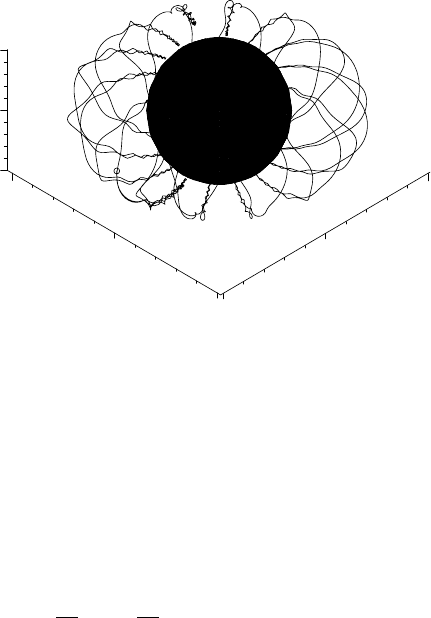
On executing the last command line and clicking on the computer plot and on

7.4. RAYLEIGH–RITZ METHOD 279

the start arrow, the motion of the proton may be viewed. The opening frame

of the animation is shown in Figure 7.6, the proton represented by the small

circle at the bottom left of the ﬁgure.

–2

–1

Figure 7.6: Path traced out by proton in the magnetic dipole ﬁeld of the earth.

In the animation, the proton spirals around the magnetic dipole ﬁeld lines, un-

dergoing repeated reﬂections in the vicinity of the poles, and precessing around

the earth. The aurora occur in the vicinity of the turning points near the poles.

7.4 Rayleigh–Ritz Method

In Chapter 1, we noted that the simple harmonic oscillator, Bessel, Legendre,

and some other commonly occuring ODEs of physical interest, are all special

cases of the Sturm–Liouville (S-L) equation,



p(x)



− q(x) y = −λw(x) y. (7.9)

for particular choices of the real functions p(x), q(x), and w(x). w(x) is taken

to be non-negative over the range x = a to b of interest. In boundary-value

problems where y satisﬁes the Sturm–Liouville boundary conditions (y or its

derivative vanish at a and b), y is the eigenfunction and λ the real eigenvalue.

The S-L equation can be formulated as a variational problem. Suppose that

we want to extremize the integral

I[y]=



[p (y



)

+ qy

] dx, subject to J[y]=



dx =1. (7.10)

The form that y must take is determined by solving the Euler–Lagrange (E-L)

equation with F = p (y



)

+ qy

− λwy

,whereλ is the Lagrange multiplier.

Substituting F into the E-L equation just yields the S-L equation, (7.9). So the

function y which makes I[y] an extremum subject to the subsidiary condition

on J[y] is an eigenfunction of the S-L equation. The Lagrange multiplier λ is

280 CHAPTER 7. CALCULUS OF VARIATIONS

the corresponding eigenvalue, while the subsidiary condition corresponds to the

normalization condition on the eigenfunctions.

Now form the quantity Λ[y]=I[y]/J[y]. Extremizing Λ is exactly equivalent

to extremizing I with the subsidiary condition on J. For S-L boundary condi-

tions, it can be shown that the value of Λ for y = y

, an eigenfunction of the

S-L equation, is equal to the eigenvalue λ

, i.e., Λ[y

]=λ

. This latter result

is the basis of the Rayleigh–Ritz method for estimating eigenvalues.

For example, for atomic or molecular systems more complicated than the

hydrogen atom, an exact analytical determination of the eigenvalues (energy

levels) and eigenfunctions is not possible, so one must resort to approximate

techniques. The Rayleigh–Ritz method is one such approach.

In this method one introduces a “trial function” φ, satisfying the boundary

conditions. For the lowest eigenvalue λ

(ground state energy for molecular

systems), it can be shown that Λ[φ] ≥ λ

, i.e., Λ provides an upper bound to

the lowest eigenvalue. By introducing one or more adjustable parameters into

φ, the estimate of λ

can usually be improved, the estimate converging on λ

from above. The Rayleigh–Ritz method can also be used to estimate higher

eigenvalues, but the estimate does not necessarily converge to the exact answer

from above. In the recipes presented here, we will only estimate the lowest

eigenvalue. The text Mathematics in Physics and Engineering by Irving and

Mullineux [IM69] deals with estimating higher eigenvalues.

7.4.1 I. M. Estimates a Bessel Zero

To arrive at a just estimate of a renowned man’s character

one must judge it by the standards of his time, not ours.

Mark Twain, American author, (1835–1910)

This recipe, provided by Ms. I.M. Curious, solves the following problem, which

has often appeared in various guises on my mathematical physics exams.

The Bessel function of order 1 satisﬁes the equation

+(k

−

=0.

Given that J

(r = 0) = 0, and noting that if we impose the boundary condition

(r = 1)=0, then k must be a zero of J

(kr), use the Rayleigh–Ritz method with

no adjustable parameters to obtain an approximate value of the ﬁrst zero of J

What is the percentage error in your answer when compared to the exact value?

Improve your estimate by including one adjustable parameter. Generally, the

agreement between the trial function and the exact solution is not nearly as

good as between the eigenvalue estimate and the exact eigenvalue. Conﬁrm

that this is the case here by plotting the trial function with one adjustable

parameter and the exact ﬁrst-order Bessel function solution.

I. M. begins by entering the general form of Λ[φ(r)]. The range of interest

here is from r = 0 to 1, so the integrals are taken to have these limits. From the

structure of Λ, she notes that the trial function need not be normalized as the

normalization constant will obviously cancel out.

7.4. RAYLEIGH–RITZ METHOD 281

restart:

Lambda:=int(p(r)*diff(phi(r),r)ˆ2+q(r)*phi(r)ˆ2,r=0..1)

/int(w(r)*phi(r)ˆ 2,r=0..1);

Λ:=



p(r)(

φ(r))

+q(r) φ(r)



w(r) φ(r)

The ﬁrst-order Bessel equation can be put into Sturm–Liouville form by choos-

ing p(r)=r, q(r)=1/r, w(r)=r, and noting that λ =k

p(r):=r: q(r):=1/r: w(r):=r:

I. M. chooses φ = r(1 − r)(1 + cr)asher

trial function, with c an adjustable

parameter which she will set to 0 in the ﬁrst part of the problem. The boundary

conditions are clearly satisﬁed, i.e., φ=0 at r =0 and 1.

phi(r):=r*(1-r)*(1+c*r):

The trial function φ is automatically substituted into Λ, which on being sim-

pliﬁed takes the following form.

Lambda:=simplify(Lambda);

Λ:=

14 (7 c

+18c + 15)

5 c

+16c +14

To answer the ﬁrst part of the question, I. M. evaluates Λ with c =0.

Lambda0:=eval(Lambda,c=0);

Λ0 := 15

Then the estimated value of k is obtained by taking the square root of Λ0.

k0:=evalf(sqrt(Lambda0));

k0 := 3.872983346

The exact (numerical) k value is obtained by using the BesselJZeros command.

kexact:=BesselJZeros(1.0,1);

kexact := 3.831705970

I. M. now calculates the percentage error, 100 (k0 − kexact)/kexact, and ﬁnds

it to be about 1.08%.

percenterror0:=((k0-kexact)/kexact)*100;

percenterror0 := 1.077258441

Now, she adjusts the parameter c to minimize the value of Λ. This is accom-

plished by calculating dΛ/dc and setting the result equal to 0.

eq:=diff(Lambda,c)=0;

eq :=

14 (14 c + 18)

5 c

+16c +14

−

14 (7 c

+18c + 15) (10 c + 16)

(5 c

+16c + 14)

Since the form of φ is deliberately not speciﬁed in the wording of the problem, I do get

a variety of possible forms submitted by my students, sometimes even trial functions that do

not satisfy the boundary conditions!

282 CHAPTER 7. CALCULUS OF VARIATIONS

Then, eq is solved for c, and put into decimal form by applying the ﬂoating

point evaluation command.

sol:=evalf(solve(eq));

sol := −0.3055081542, −1.785400936

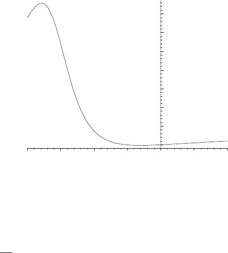
Two values are generated for c. To decide on which value will minimize Λ, I. M.

plots Λ over the range c= −2 to 1. The resulting picture is shown in Figure 7.7.

plot(Lambda,c=-2..1,labels=["c","Lambda"]);

Lambda

–2 –1 0

Figure 7.7: Λ versus c.

From the ﬁgure, the value c −1.79 must be ruled out as then Λ  50 > Λ0.

Λ should be evaluated with c −0.31. This is done in Λ1, the number being

slightly lower than Λ0= 15.

Lambda1:=eval(Lambda,c=sol[1]);

Λ1 := 14.84137598

Then, k1 =

√

Λ1 is calculated and the percentage error determined once again.

k1=sqrt(Lambda1);

k1 := 3.852450646

percenterror:=((k1-kexact)/kexact)*100;

percenterror := 0.5413952992

With one adjustable parameter included, the estimated value of k, i.e., k1 ,now

only diﬀers by 0.54% from the exact value. The corresponding trial function is

given by φ1.

phi1:=eval(phi(r),c=sol[1]);

φ1:=r (1 − r)(1− 0.3055081542 r)

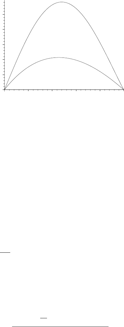
Toﬁnishtheproblem,I.M.plotsφ1 and the exact Bessel solution in Fig. 7.8.

plot([phi1,BesselJ(1,kexact*r)],r=0..1,color=[red,blue],

labels=["r","phi"]);

7.4. RAYLEIGH–RITZ METHOD 283

0.1

0.2

0.3

0.4

0.5

phi

0.2 0.4

0.6

0.8 1

Figure 7.8: Comparison of trial function (lower curve) and exact solution (top).

She observes that although the estimated value of k is extremely good, the trial

function φ1 doesn’t do a very good job of representing the exact ﬁrst-order

Bessel function solution over the range r = 0 to 1. Part of the discrepancy could

be due to the fact that φ1andJ

are not similarly normalized.

7.4.2 I. M. Estimates the Ground State Energy

The only diﬀerence between a tax man and a taxidermist

is that the taxidermist leaves the skin.

Mark Twain, American author, (1835–1910)

In the last example, the trial function contained one adjustable parameter.

In the following problem, for which I. M. Curious will provide her recipe as a

solution, there are two parameters which must be adjusted to minimize Λ.

Use the Rayleigh–Ritz procedure and the trial function φ = e

−x

to esti-

mate the ground state energy E

of a particle satisfying the one-dimensional

Schr¨odinger equation (in appropriate units)

− x

ψ = −Eψ, −∞ <x<∞.

Improve your estimate by considering φ = e

−x

(1 + c1 x

+ c2 x

), with two

adjustable parameters c1 and c2 .

I. M. enters the general form of Λ, the range now from x=−∞ to ∞.

restart: with(plots):

Lambda:=int(p(x)*diff(phi(x),x)ˆ2+q(x)*phi(x)ˆ2,x=-infinity

..infinity)/int(w(x)*phi(x)ˆ 2,x=-infinity..infinity);

Λ:=



∞

−∞

p(x)(

φ(x))

+q(x) φ(x)



∞

−∞

w(x) φ(x)

284 CHAPTER 7. CALCULUS OF VARIATIONS

From the given ODE, she identiﬁes p(x)=1, q(x)=x

,andw(x)=1, which are

now entered. The eigenvalue λ= E.

p(x):=1: q(x):=xˆ4: w(x):=1:

I. M. enters the trial wave function with the two adjustable parameters. The

ﬁrst part of the question can be answered by setting c1 =0, c2 =0.

phi(x):=exp(-xˆ2)*(1+c1*xˆ2+c2*xˆ4);

φ(x):=e

(−x

)

(1 + c1 x

+ c2 x

)

φ(x) is automatically substituted into Λ, which on simplifying is as follows.

Lambda:=simplify(value(Lambda));

Λ:=

13995 c2

+ 10248 c2 c1 − 1248 c2 + 3472 c1

+ 4864 − 128 c1

16 (256 + 105 c2

+ 120 c2 c1 + 128 c1 +96c2 +48c1

)

The estimate of the ground state energy with no adjustable parameters is de-

termined in Λ0.

Lambda0:=evalf(eval(Lambda,{c1=0,c2=0}));

Λ0 := 1.187500000

So, I. M. estimates the ground state energy E

to be about 1.19 units. Now,

she considers the situation when the parameters are non-zero. In this case, she

must minimize Λ with respect to both parameters. This is done by imposing

the conditions ∂Λ/∂c1 =0 and ∂Λ/∂c2 =0, which is done in C1 and C2 .

C1:=simplify(diff(Lambda,c1))=0;

C2:=simplify(diff(Lambda,c2))=0;

C1 := −2(−68352 c2 + 18855 c2

+ 19200 c2

c1 − 24576 c2 c1

+ 20976 c2

+ 2352 c2 c1

− 40960 c1 − 14080 c1

+ 20480)

/(256 + 105 c2

+ 120 c2 c1 + 128 c1 +96c2 +48c1

)

C2 := 6(64000 c2 + 6285 c2

c1 + 37600 c2 c1 + 15360 c2

+ 6400 c2 c1

+ 19712 c1 + 9728 c1

+ 784 c1

− 8192)

/(256 + 105 c2

+ 120 c2 c1 + 128 c1 +96c2 +48c1

)

The formidable nonlinear algebraic equations C1 and C2 must be numerically

solved for c1 and c2. To guide her in arriving at the correct solution, I. M. forms

a functional operator gr to apply the implicitplot command to a speciﬁed

algebraic equation A, the color of the curve being dictated by the choice of B.

To obtain smooth curves, the number of plotting points is increased to 2000.

gr:=(A,B)->implicitplot(A,c1=-10..10,c2=-10..10,

numpoints=2000,color=B):

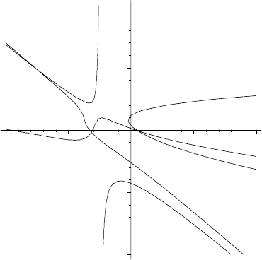
Aplotofc2 versus c1 satisfying the equation C1 follows on taking A= C1 in

gr. The curve will be colored blue. Similarly, a green curve is generated for the

choice A = C2 . The two curves are superimposed with the display command,

the resulting picture being shown in Figure 7.9.

display({gr(C1,blue),gr(C2,green)});

7.4. RAYLEIGH–RITZ METHOD 285

–10

–5

–10

–5 5

Figure 7.9: Possible values of c1 and c2 occur at intersection points.

Within the range of the plot, I. M. spots three intersection points. Applying

the ﬂoating point solve command to C1 and C2 without specifying the search

range for c1 and c2 ,

s1:=fsolve({C1,C2},{c1,c2});

s1 := {c1 = −7.524875339, c2 =4.879077669}

yields the intersection point in the second quadrant of Figure 7.9. To obtain

the other two intersection points, I. M. now speciﬁes the appropriate plotting

ranges in the fsolve command in s2 and s3

s2:=fsolve({C1,C2},{c1,c2},{c1=0..2,c2=-2..2});

s2 := {c1 =0.5221933646, c2 = −0.05771753990}

s3:=fsolve({C1,C2},{c1,c2},{c1=-5..0,c2=-2..2});

s3 := {c2 = −0.2086941568, c1 = −3.169995132}

An operator L is created to evaluate λ for a speciﬁed s, which I. M. then applies

to s1 , s2 ,ands3 in Λ1, Λ2, and Λ3.

L:=s->eval(Lambda,s):

Lambda1:=L(s1); Lambda2:=L(s2); Lambda3:=L(s3);

Λ1 := 16.71552532 Λ2 := 1.061092905 Λ3 := 7.535881788

The estimates Λ1 and Λ3 are rejected as both are larger than Λ0  1.19. The

estimate Λ2  1.06 is lower than Λ0, so represents an improved estimate of

the ground state energy. It would appear from Iam’s recipe that her estimates

are converging on the value E

=1. Itisleftasanexerciseforyoutoconﬁrm

whether this conclusion is correct or not.

286 CHAPTER 7. CALCULUS OF VARIATIONS

7.5 Supplementary Recipes

07-S01: Geodesic

The curve of shortest length joining two points is called a geodesic. Show that

the geodesic on the surface of a right circular cylinder of radius a is a helix. Plot

the geodesic on a cylinder of radius a =2 between the points (z =1/2,θ=π/8)

and (5/2,π/2), where z is the cylinder axis coordinate and θ the polar angle.

07-S02: Laws of Geometrical Optics

Use Fermat’s principle to prove the following geometrical optics relations:

(a) A light ray incident at an angle i to the normal on a planar mirror is

reﬂected back into the same medium at an angle r



= i to the normal.

(b) Consider a light ray traveling from a medium with refractive index n

through a planar interface into a medium with refractive index n

.If

the light ray is incident at an angle i, the angle of refraction r in the

second medium is given by Snell’s law: n

sin i = n

sin r. Both angles

are measured with respect to the normal to the interface.

07-S03: Bending of Starlight

According to the theory of general relativity, the trajectory of starlight travel-

ing in the spherically symmetric static ﬁeld of the sun is such as to minimize

the integral

I =





(dr/γ)

+(rdθ)

/γ

where (r, θ) are polar coordinates and γ =1−(2 Gms)/(c

r), G being the grav-

itational constant, ms the mass of the sun, and c the vacuum speed of light.

Using the variational approach and setting u =1/r, prove that the diﬀerential

equation of the trajectory can be written in the form

dθ

+ au= bu

where a and b remain to be identiﬁed. Taking G=6.673×10

−11

N·m

/kg

, ms=

1.99×10

kg, c =2.997×10

m/s, and the sun’s radius Rs=6.96×10

m, numer-

ically solve the nonlinear ODE for u(θ), taking u(0)= 1/(10Rs)anddu(0)/dθ =

0. Then use the spacecurve command to plot (r(θ) cos(θ),r(θ)sin(θ)) for

θ = −π/2toπ/2. Include the sun in your ﬁgure.

07-S04: Another Refractive Index

Using Fermat’s principle, prove that light rays in a medium with refractive

index n(x, y)=1/y will follow a path which is the arc of a circle.

07-S05: Mirage

Assuming that the refractive index varies linearly with height in the following

way, n(x, y)=n

(1 + αy)withn

> 0andα>0, use Fermat’s principle to

determine the angle θ by which a point P is apparently lowered when viewed

from a point P



at the same height as P at a horizontal distance d.The

parameter α is suﬃciently small that you may take αd<< 1. This problem is

relevant to the phenomenon of mirages observed in hot desert regions.

7.5 SUPPLEMENTARY RECIPES 287

07-S06: A Constrained Extremum

Determine a function y(x) for which I =



((y



)

− y

) dx is an extremum,

subject to N =



ydx=1, and y(0) =0, y(π) =1. Plot y(x).

07-S07: Maximum Volume

Find the maximum value of the volume V = xyz, subject to the condition

+ y

+ z

=1, with a, b,andc positive. Use (a) the direct method,

(b) the Lagrange multiplier method.

07-S08: Eigenvalue Estimate

Taking a trial function of the form y =A

+ A

x + A

+ A

, estimate the

smallest eigenvalue k of y



+ k

y = 0, subject to y(0) = y(1) = 0. Compare the

estimate and the trial function with the exact results.

07-S09: Surface of Revolution

Consider a surface of revolution generated by revolving a curve y(x) about the

x-axis. The curve is required to pass through the ﬁxed end points (x=0,y=1)

and (x =1,y= 2). Determine what shape y(x)musthavesothattheareaof

the resulting surface will be a minimum. Plot the curve.

07-S10: Dido Wasn’t a Dodo

Given a closed planar curve C of a ﬁxed length L, what shape should the curve

have to maximize the enclosed area A? The answer, known as the isoperimetric

theorem, is a circle. Evidently, this theorem has been known from about 900

BC, and according to Virgil’s Aneid was applied by Queen Dido in a practical

way to establish the city of Carthage (now Tunisia) in North Africa. The

local ruler, King Jambas, agreed to sell her all the land that she could enclose

within a bull’s hide. She cleverly had the hide cut into thin strips which were

joined end to end to form a long “string” and made use of a variation on the

isoperimetric theorem. She cleverly maximized A by selecting a straight portion

of the Mediterranean coast and laying the string out in a semicircle with the

string’s two ends touching the coast.

Given that A =



(xdy− ydx) for a closed planar curve C, make use of

the Euler–Lagrange equation to prove the isoperimetric theorem.

07-S11: Another Approach to the String Equation

In recipe 04-1-1, the wave equation for small transverse vibrations of a light

ﬂexible horizontal string under tension and ﬁxed on its ends was derived us-

ing Newton’s second law of motion. Another approach to deriving the wave

equation is to use the variational method.

It can be shown that a necessary condition for y =y(x, t)tobeanextremal



F (x, t, y, y

) dx dt is

∂F

∂y

−

∂

∂x



∂F

∂y



−

∂

∂t



∂F

∂y



=0.

Here y

≡ ∂y/∂x, y

≡ ∂y/∂t, x

and x

are ﬁxed end points, and t

and t

are

speciﬁed times. Making use of this extension of Lagrange’s equation, derive the