Enns R.H. Computer Algebra Recipes for Mathematical Physics

Подождите немного. Документ загружается.

8.1. NONLINEAR ODES: EXACT METHODS 299

plot(T,A=0..5,labels=["A","T"],view=[0..5,0..2*Pi]);

1234

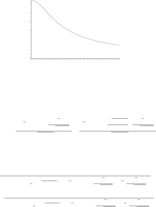
Figure 8.3: Period T of the hard spring versus amplitude A.

Unlike the situation for a linear spring, the period of the hard spring is ampli-

tude dependent, decreasing with increasing values of A. To determine x(t), the

integral t=



−A

(1/eq5 ) dy is evaluated assuming that A>0andx>−A.

eq6:=t=int(1/eq5,y=-A..x) assuming A>0,x>-A;

eq6 := t =

√

2 EllipticK(

√

2 A

√

1+A

)

√

2+2A

−

√

2 EllipticF(

√

− x

√

2 A

√

1+A

)

√

2+2A

eq6 is now solved for x, which produces positive and negative square root ex-

pressions, which are assigned the names x1 and x2 . Both solution branches will

be needed to plot the complete oscillation of the hard spring.

eq7:=solve(eq6,x); x1:=eq7[1]; x2:=eq7[2];

x1 :=



1− JacobiSN(

√

2+2A

− 2

√

2 EllipticK(

√

1+A

))

√

2 A

√

1+A

)

x2 :=

−



1−JacobiSN(

√

2+2A

−2

√

2 EllipticK(

√

2 A

√

1+A

))

√

2 A

√

1+A

)

The “special” function JacobiSN appearing in the output is the Jacobi elliptic

sine function. Setting u ≡ F (φ\α), φ is referred to as the “amplitude” of u,

written as φ =amu. The elliptic sine function is deﬁned as sn u = sin(am u)=

sin φ. The Maple command for numerically calculating sn u for a given m value

is evalf(JacobiSN(u,sqrt(m))). The reader is referred to Abramowitz and

Stegun [AS72] for the properties of the elliptic functions.

300 CHAPTER 8. NLODES & PDES OF PHYSICS

To plot the hard spring solution, let’s choose a speciﬁc value of the ampli-

tude, say A=3. The period T1 is ﬁrst evaluated

T1:=evalf(eval(T,A=3));

T1 := 2.294401860

and then a piecewise function x is created, using x1 for t<T1 /4, x2 for

T1 /4 <t<3T1 /4, and so on.

x:=piecewise(t<T1/4,x1,t<3*T1/4,x2,t<5*T1/4,x1,

t<7*T1/4,x2,t<9*T1/4,x1,t<11*T1/4,x2):

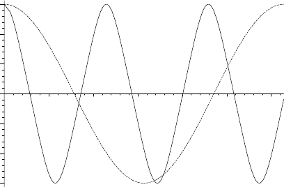
Then x is evaluated at A =3 and plotted along with the solution 3 cos(t)tothe

corresponding linear spring equation, the result being shown in Figure 8.4.

plot([eval(x,A=3),3*cos(t)],t=0..2*Pi,color=[red,blue],

linestyle=[1,3],labels=["t","x"]);

–3

1234

Figure 8.4: Solid curve: hard spring; Dashed curve: linear spring (a= 0).

As expected, the hard spring oscillates more rapidly than the linear spring.

8.2 Nonlinear ODEs: Graphical Methods

Two recipes are presented which illustrate how a second-order NLODE, or a

system of two ﬁrst-order equations, can be graphically solved and interpreted.

8.2.1 Joe and the Van der Pol Scroll

Sometimes one likes foolish people for their folly,

better than wise people for their wisdom.

Elizabeth Gaskell, English novelist, (1810–65)

This recipe is inspired by my reminiscences of a former student in my non-

linear physics class, whose identity I will protect by calling him “Joe”. In class,

8.2. NONLINEAR ODES: GRAPHICAL METHODS 301

I had derived the “equation of motion” for a tunnel diode electrical circuit, the

ODE taking the form of the nonlinear Van der Pol (VdP) equation,

¨x + (x

− 1) x + x =0, (8.6)

where x is related to the voltage change across the diode and the positive

parameter  depends on certain circuit parameters. From a mechanical view-

point, the VdP equation follows on applying Newton’s second law to a unit

mass which experiences a Hooke’s law restoring force, F

Hooke

=−x,andadrag

force, F

drag

=− (x

−1) ˙x.For=0, Eq. (8.6) reduces to the simple harmonic

oscillator equation which has undamped oscillatory solutions. For >0, the

drag force has a rather peculiar property. For x>1and ˙x>0, F

drag

< 0, which

tends to reduce the size of the oscillations, but for x<1and ˙x still positive,

drag

> 0, and the oscillations tend to grow in amplitude. In the tunnel diode

case, it is the latter feature which causes the diode to begin to spontaneously

oscillate even if it is connected to a steady (non-oscillatory) power supply.

As a follow up to the class room derivation, I had then asked the class

to solve the VdP equation for  = 5 for a few initial conditions of their own

choosing, using a graphical/numerical technique called the method of isoclines.

The basis of the isoclines method is as follows. Setting y ≡ ˙x, the second-order

VdP equation can be reduced to a system of two coupled ﬁrst-order ODEs, viz.,

˙x = y, ˙y =  (1 − x

) y − x. (8.7)

Since the time doesn’t explicitly appear

in (8.7), it may be eliminated by form-

ing the ratio dy/dx =((1−x

) y −x)/y. But this ratio is just the slope tangent

to the solution “trajectory” in the x-y plane (called the phase plane)atanin-

stant in time. A tangent ﬁeld picture can be created by drawing systematically

spaced arrows in the x-y plane, the arrows oriented along the slope directions

and the arrow heads pointing in the direction of increasing time. Given some

initial condition, x(0), y(0), the solution curve (called a phase-plane trajectory)

can be drawn in the x-y plane by following the arrows. A tangent ﬁeld picture

with one or more superimposed solution curves is referred to as a phase-plane

portrait of the autonomous ODE or ODE system.

The method of isoclines was commonly used in the pre-computer age to sys-

tematically draw the tangent ﬁeld arrows. In this method, curves corresponding

to diﬀerent constant slopes (the isoclines) were drawn and equally spaced ar-

rows pointing in the slope direction placed on each isocline. Once the x-y plane

was ﬁlled with a suﬃciently ﬁne grid of arrows, one could see how a solution

would evolve with time from any point in the phase plane.

So, why do I remember Joe? It’s because when Joe handed in his solution

to the problem (a week late!), it was in the form of a large cylindrical scroll

fastened with an elastic band. Removing the band, I began to unwind the

scroll. To my amazement, I found that the scroll stretched across the width of

my oﬃce. Joe had evidently chosen the wrong scale for his initial conditions and

stubbornly kept splicing sheets together until he obtained a complete solution

The equations are referred to as autonomous.

302 CHAPTER 8. NLODES & PDES OF PHYSICS

trajectory. To compound Joe’s woes, he had not written a simple program to

automate the process but had evidently used a calculator and then plotted the

isoclines, arrows, and trajectories completely by hand. However, to his credit,

the plot was basically correct and I didn’t have the heart to penalize Joe for

handing the problem in late.

The following recipe carries out the solution to Joe’s problem painlessly

and quickly. It makes use of the phaseportrait command which is in Maple’s

DEtools library, so this package is loaded. I will take =5.

restart: with(DEtools): epsilon:=5:

Equations (8.7) are entered in ode1 and ode2 .

ode1:=diff(x(t),t)=y(t);

ode1 :=

x(t)=y(t)

ode2:=diff(y(t),t)=epsilon*(1-x(t)ˆ2)*y(t)-x(t);

ode2 :=

y(t)=5(1− x (t)

) y(t) − x(t)

Two initial conditions are considered. The phase-plane trajectory will start

from near the origin for ic1 , and reasonably far from the origin for ic2 .

ic1:=x(0)=0.01,y(0)=0.01: ic2:=x(0)=-1,y(0)=6:

The following phaseportrait command is used to plot the tangent ﬁeld

and

the two trajectories corresponding to the above initial conditions. In the argu-

ment, the two ODEs are entered as a list, as are the dependent variables to be

solved for. The time range is taken to be t = 0 to 20 for the solution curves

and the initial conditions are entered as a list of lists. The plot range is taken

to be x = −2.5to2.5,andy = −10 to 13. To obtain accurate solution curves,

the numerical step size is taken to be 0.01. The dirgrid option controls the

number of tangent arrows to be drawn. Here, I have chosen to plot 30 × 30=900

arrows. The default is 20 × 20. Various arrow styles are available. I have cho-

sen arrows=MEDIUM and colored the arrows blue. Finally, the two trajectories

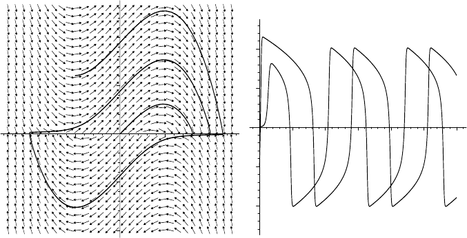
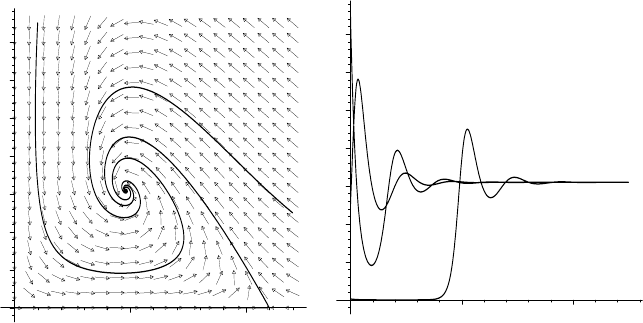
are colored red and green. The result is shown on the left of Figure 8.5.

phaseportrait([ode1,ode2],[x(t),y(t)],t=0..20,[[ic1],[ic2]],

x=-2.5..2.5,y=-10..13,stepsize=.01,dirgrid=[30,30],

arrows=MEDIUM,color=blue,linecolor=[red,green]);

The tangent arrows provide a visual guide to how trajectories will evolve as the

time increases. As time evolves, the trajectory corresponding to ic1 unwinds

in a spiral fashion from near the origin onto a closed loop, indicative of a cyclic

solution. The trajectory corresponding to ic2 winds onto the same closed loop.

In fact, no matter what the initial conditions, all trajectories wind onto the

closed loop, which is an example of a limit cycle. In fact, since all trajectories

wind onto it as t →∞,itisreferredtoasastable limit cycle.

By including the option scene=[t,x(t)],thephaseportrait command

can also be used to plot x(t) versus t.

Isoclines are not drawn.

8.2. NONLINEAR ODES: GRAPHICAL METHODS 303

–10

–2 2

–2

x(t)

Figure 8.5: Left: trajectories winding onto limit cycle. Right: x(t) versus t.

phaseportrait([ode1,ode2],[x(t),y(t)],t=0..30,[[ic1],[ic2]],

x=-2.5..2.5,y=-10..13,stepsize=.01,scene=[t,x(t)],

linecolor=[red,green]);

The result is shown on the right of Figure 8.5. After a transient interval, the

two curves have identical shapes. The steady-state curves are characterized

by periods of relatively slowly varying x, periodically interspersed with abrupt

changes. These types of oscillations are referred to as relaxation oscillations.

By increasing , the period of the oscillations can be increased.

8.2.2 Squid Munch (Slurp?) Herring

Man is the only animal that can remain on friendly terms with the

victims he intends to eat until he eats them.

Samuel Butler, English author, (1835–1902)

Another pre-computer approach to qualitatively sketching possible solution

curves of a second-order autonomous nonlinear ODE (or two coupled ﬁrst-

order NLODEs) in the phase-plane was to ﬁrst locate all the stationary or

singular points (where all derivatives vanish) of the nonlinear ODE, identify

their “topological” nature, and use this knowledge to sketch the trajectories.

More speciﬁcally, this topological approach is as follows.

Consider the pair of ﬁrst-order autonomous ODEs,

˙x = P (x, y), ˙y = Q(x, y), (8.8)

where, in general, P and Q are nonlinear functions and we have taken time

as the independent variable. For the Van der Pol oscillator of the last recipe,

P ≡ y and Q ≡−x +  (1 − x

) y. A stationary point (x

, y

) corresponds to

304 CHAPTER 8. NLODES & PDES OF PHYSICS

˙x =0 and ˙y =0, or P (x

)=Q(x

) = 0. For the Van der Pol oscillator,

there is only one stationary point, namely (x

=0, y

= 0), i.e., the origin. For

any ordinary point outside a stationary point, we can write its coordinates as

x=x

+ u, y = y

+ v. The slope of the trajectory at an ordinary point is

Q(x

+ u, y

+ v)

P (x

+ u, y

+ v)

. (8.9)

For an ordinary point close to a stationary point, the numerator and denomi-

nator on the rhs can be Taylor expanded about (x

)inpowersofu and v,so

cu+ dv+ ···

au+ bv+ ···

, (8.10)

where a ≡ (∂P/∂x)

, b ≡ (∂P/∂y)

, c ≡ (∂Q/∂x)

, d ≡ (∂Q/∂y)

Provided that bc− ad = 0, the trajectories near the stationary point can be

correctly described by retaining only the linear terms in u and v in (8.10). In

this case, the stationary point is referred to as simple. In this approximation,

equation (8.10) can be thought of as resulting from the pair of linear ODEs,

˙u = au+ bv, ˙v = cu+ dv, (8.11)

which have solutions of the form (u, v) ∼ e

λt

,withλ=−



− 4 q,where

p = −(a + d)andq = ad− bc. Detailed examination of the two λ roots reveals

that there are only four types of simple stationary points, the saddle, focal or

spiral, nodal,andvortex points. Which type occurs depends on the ranges of q,

p,andp

− 4 q as indicated in Table 8.1.

Stationary Point q=a d–b c p=–(a+d) p

–4q

saddle < 0

≥ 0and≤ 0 > 0

higher order

=0 ≥ 0and≤ 0 ≥ 0

stable focal > 0 < 0

stable nodal > 0 ≥ 0

vortex or focal > 0 =0 < 0

unstable focal < 0 < 0

unstable nodal < 0 ≥ 0

Table 8.1: Classiﬁcation of stationary or singular points.

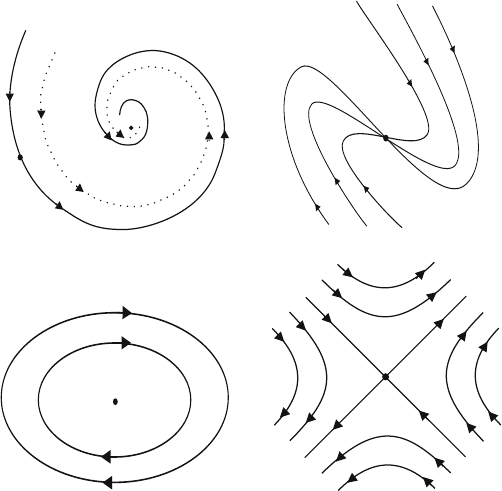
In the neighborhood of these simple stationary points, the trajectories have

the schematic form shown in Figure 8.6, the arrows indicating increasing time.

Stable focal and nodal points are shown, the trajectories approaching the sta-

tionary points as t →∞.Forunstable focal and nodal points, the arrow direc-

tions are reversed. The origin of the phase-plane for the Van der Pol oscillator

is an example of an unstable focal point, which can be seen in Figure 8.5.

For q>0andp = 0, note that either a vortex or focal point occurs. The

reason for the “uncertainty” is that inclusion of quadratic (or higher) terms in

8.2. NONLINEAR ODES: GRAPHICAL METHODS 305

Figure 8.6: Curves near a focal (F ), nodal (N), vortex (V ), saddle (S) point.

the Taylor expansion may turn a closed loop (for the vortex) into a spiral. In-

stead of examining these higher-order terms, we quite often rely on a suﬃcient,

but not necessary, global theorem due to Poincar´e, which is built on symme-

try considerations. If P (x, −y)=−P (x, y) and Q(x, −y)=Q(x, y), then the

stationary point is a vortex, not a focal point.

For q = 0 and arbitrary p, the stationary point is no longer simple, and is

referred to as a higher-order stationary point. Trajectories in the neighborhood

of these points tend to be more complicated than in Figure 8.6.

In the pre-computer age, we would locate and identify the stationary points

and attempt to draw the trajectories in the entire phase-plane by splicing the

trajectories around each stationary point together. This procedure works well

enough when the nonlinear ODE has only a few widely separated simple sta-

tionary points, with no higher-order points or limit cycles present. But in this

computer age, we can simply use, e.g., the phaseportrait command. However,

it’s still important to know the locations and types of stationary points as this

provides a deeper understanding of the solution curves. This is illustrated in

the following mathematical biology example.

The major food source for squid is herring. If S and H arethenumbersof

squid and herring, respectively, per acre of seabed, the interaction between the

two species can be modeled [Sco87] by the system (with time in years)

H = k

H − k

− k

HS,

S = −k

S − k

+ k

HS, (8.12)

306 CHAPTER 8. NLODES & PDES OF PHYSICS

with k

=1.1, k

=10

−5

, k

=10

−3

, k

=0.9, k

=10

−4

,andk

=2×

−5

. The ﬁrst term on the rhs of

H represents the natural growth of the

herring population if the resources (food) were unlimited, the second term limits

the growth because of the ﬁnite resources, and the third term represents the

decrease in population due to interaction (i.e., being eaten) with the squid. You

should be able to interpret the terms in the other equation.

(a) Locate and classify all the stationary points of the NLODEs. Plot the

tangent ﬁeld and show the trajectories for (i) H(0) = 5, S(0) = 5; (ii)

H(0) = 10000, S(0) = 1500; (iii) H(0) = 120000, S(0) = 500. Take t =0 to

50. Relate the results to the stationary points.

(b) Suppose that every squid was removed from the area occupied by the

herring and from all surrounding areas. Would H increase indeﬁnitely

or would it approach an upper limit? If you believe the latter would

occur, what is that number? If the squid free situation had persisted for

many years, what are S and H two years later if a pair of fertile squid is

introduced into the area? Round the numbers to the nearest integer.

The DEtools library package is needed for the phaseportrait command.

restart: with(plots): with(DEtools):

The coeﬃcient values are entered,

k1:=1.1: k2:=10ˆ(-5): k3:=10ˆ(-3): k4:=0.9: k5:=10ˆ(-4):

k6:=2*10ˆ(-5):

and functional operators P and Q introduced to generate the rhs of the NLODEs

(8.12) for arbitrary H and S.

P:=(H,S)->k1*H-k2*Hˆ2-k3*H*S; Q:=(H,S)->-k4*S-k5*Sˆ2+k6*H*S;

P := (H, S) → k1 H − k2 H

− k3 HS

Q := (H, S) →−k4 S − k5 S

+ k6 HS

Using P and Q, the necessary derivatives to calculate a, b, c, d are calculated.

These expressions have to be evaluated at each stationary point.

a:=diff(P(H,S),H); b:=diff(P(H,S),S); c:=diff(Q(H,S),H);

d:=diff(Q(H,S),S);

a:= 1.1 −

50000

−

1000

b:= −

1000

c :=

50000

d:= −0.9 −

5000

50000

The number of stationary points and their coordinates is determined by setting

P (H, S)=0 and Q(H, S)= 0 and solving for H and S.

sol:=solve({P(H,S)=0,Q(H,S)=0},{H,S});

sol := {H =0., S =0.}, {H = 110000., S =0.}, {H =0., S = −9000.},

{S = 619.0476190,H= 48095.23810}

The NLODEs have four stationary points at the locations indicated above. Note

that the stationary point at H =0, S = −9000 is in a non-physical portion of

the phase-plane, since we must have H ≥ 0andS ≥ 0.

8.2. NONLINEAR ODES: GRAPHICAL METHODS 307

Functional operators p and q are now formed to calculate p= −(a + d)and

q = ad− bc for the ith stationary point.

p:=i->evalf(eval(-(a+d),sol[i])):

q:=i->evalf(eval(a*d-b*c,sol[i])):

In the following do loop, p, q,andr ≡ p

− 4 q are calculated for each of the

four singular points. The classiﬁcation scheme of Table 8.1 is implemented by

using a conditional if...then...elif...else...end if statement. elif is

a contraction of “else if”. This allows each singular point to be classiﬁed. For

this conditional statement to work, numerical (not symbolic) values must be

provided for the coeﬃcients in the NLODEs.

forifrom1to4do

sol[i]; p||i:=p(i); q||i:=q(i); r||i:=simplify(p||iˆ2-4*q||i);

if q||i<0 then s||i:=saddle;

elif q||i>0 and p||i>0 and r||i<0 then s||i:=stablefocal;

elif q||i>0 and p||i>0 and r||i>=0 then s||i:=stablenodal;

elif q||i>0 and p||i<0 and r||i<0 then s||i:=unstablefocal;

elif q||i>0 and p||i<0 and r||i>=0 then s||i:=unstablenodal;

elif q||i>0 and p||i=0 then sing||i:=vortex

or focal;

else s||i:=higherorder; end if: s||i;

end do;

{H =0., S =0.} p1:= −0.2000000000 q1:= −0.9900000000

r1:= 4. saddle

{H = 110000., S =0.} p2:= −0.2000000000 q2:= −1.430000000

r2:= 5.760000000 saddle

{H =0., S = −9000.} p3:= −11. q3:= 9.090000000

r3:= 84.64000000 unstablenodal

{H = 48095.23810,S= 619.0476190} p4:= 0.5428571428 q4:= 0.6252380953

r4:= −2.206258504 stablefocal

So, the stationary points at H =0, S = 0 and

H = 110, 000, S = 0 are saddle

points, H =0, S = −9000 is an unstable nodal point, and H  48095, S 619 is

a stable focal point. This implies that all trajectories in the “physical region”

H ≥ 0, S ≥ 0 will be attracted to the stable focal point as t →∞. I.e., if the

equations are valid for all t (which they wouldn’t be!), one would ultimately

end up with about 48095 herring and 619 squid per acre of seabed. To conﬁrm

this, let’s create a phase-plane portrait, ﬁrst entering the NLODE system.

sys:=diff(H(t),t)=P(H(t),S(t)),diff(S(t),t)=Q(H(t),S(t));

sys :=

H (t)=1.1 H (t) −

100000

H (t)

−

1000

H (t) S (t),

S(t)=−0.9 S (t) −

10000

S(t)

50000

H (t) S (t)

308 CHAPTER 8. NLODES & PDES OF PHYSICS

A functional operator PP is formed to generate the phase-plane portrait S(t)

vs. H(t), as well as H(t)vs.t and S(t)vs. t, for the system of NLODEs.

PP:=(X,Y)->phaseportrait([sys],[H(t),S(t)],t=0..50,

[[H(0)=5,S(0)=5],[H(0)=10000,S(0)=1500],

[H(0)=120000,S(0)=500]],stepsize=.05,scene=[X,Y],

arrows=MEDIUM,color=blue,dirgrid=[20,20],

linecolour=[red,green,black],xtickmarks=3):

Which plot is produced depends on the choice of scene variables X and Y.The

lists of equations and dependent variables are entered as arguments, along with

the time range which is taken here to be 0 to 50 years. The initial population

numbers are given as a list of lists. The numerical time stepsize is taken to

be 0.05 years and medium blue arrows are chosen for the tangent ﬁeld. The

grid density for the tangent arrows is taken to be 20 × 20. The trajectories

corresponding to the three initial conditions are colored red, green, and black,

and the number of tickmarks along the horizontal axis controlled.

Then PP is used to produce the phase-plane portrait, as well as plots of H(t)

versus t and S(t) versus t.

PP(H(t),S(t)); PP(t,H(t)); PP(t,S(t));

600

1200

S(t)

50000

100000

H(t)

600

1200

S(t)

20 40

Figure 8.7: Phase-plane portrait (left) and S vs. t (right) for 3 initial conditions.

S vs. H is shown on the left of Figure 8.7, and S vs. t on the right. In the

phase-plane picture on the left, one can clearly see that all three trajectories

asymptotically wind onto the stable focal point, as was anticipated. The trajec-

tory corresponding to H(0)= 5, S(0) =5 initially travels horizontally very close

to the H(t) axis until it gets close to the saddle point at S =0, H =110, 000. It

then makes an abrupt turn, heading towards the stable focal point and winding

onto it. The trajectory starting at H(0) =10, 000, S(0)= 1500 initially descends

almost vertically until it begins to follow the tangent ﬁeld in the vicinity of the