Enns R.H. Computer Algebra Recipes for Mathematical Physics
Подождите немного. Документ загружается.

6 INTRODUCTION
By inspecting the figure, we can see that the maximum velocity occurs around
the 5 s mark and is about 24 m/s. A slightly more accurate estimate can be
obtained by placing the cursor on the top of the tallest peak in the computer
picture and clicking the mouse. The horizontal and vertical coordinates of
the cursor location are displayed in a small viewing box at the top left of
the computer screen. A much more accurate answer follows on setting the
acceleration A equal to zero and applying the floating point solve (fsolve)
command in a time range which includes the tallest peak, say t = 4 to 6 s. This
yields an answer T2 for the time to 10 digits, Maple’s default accuracy.
>
T2:=fsolve(A=0,t=4..6);
T2 := 4.868771376
The maximum velocity occurs at T2 4.87 seconds. Then, using the eval
command to evaluate V at t = T2 ,
>
Vmax:=eval(V,t=T2);
Vmax := 23.81789390
yields a maximum velocity Vmax 23.8m/s. Theconvert command with the
units option is used to convert Vmax from m/s to km/h.
>
Vmax:=convert(Vmax,units,m/s,km/h);
Vmax := 85.74441804
The maximum velocity is 85
3
4
km/h, which doesn’t seem excessively high.
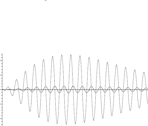
What about the acceleration? Let’s plot A and V together in the same figure
over the time range t =0toT/2 = 10 seconds. Two plot options (color and
linestyle) are introduced. A red solid line is chosen for V , a blue dashed line
for A. Note that V and A as well as the options have been entered as “Maple
lists” (the elements separated by commas and enclosed in square brackets).
Maple preserves the order and repetition of elements in a list.
>
plot([V,A],t=0..T/2,color=[red,blue],linestyle=[SOLID,DASH]);
–200
–100
0
100
200
24
6
810
t
Figure 2: A (dashed curve) and V (solid) versus time t.

INTRODUCTORY RECIPES 7
If you are printing pictures with multiple plots in black and white, it is partic-
ularly important to control the line style so the curves can be distinguished.
In Figure 2, we can clearly see that the acceleration is a maximum when
the velocity is zero and zero when the velocity is a maximum. The maximum
acceleration is over 200 m/s
2
. Since the acceleration due to gravity is about 10
m/s
2
, this corresponds to roughly 20 “Gees”. Do you think that such an ac-
celeration is possibly dangerous? Justify your answer. Perhaps, do an Internet
search on the effects of rapid acceleration on the human body.
Next, we look at a two-dimensional kinematics example which introduces
you to the use of a Maple library package. Library packages are very important
because they save you the effort of programming specialized plotting and math-
ematical operations. Approximately 90% of Maple’s mathematical knowledge
resides in the Maple library. Most of the recipes in this text use one or more
library packages.
D.2 The Patrol Route of Bertie Bumblebee
Belief like any other moving body follows the path of least resistance.
Samuel Butler, British author, (1835–1902)
Bertie Bumblebee, intrepid sentry for the central bee hive on the terraformed
planet Erehwon
1
, flies on a patrol route described t minutes after leaving the
central hive by the radial coordinate r(t)=at
2
e
−bt
/(1 + t
2
)sretem(aunitof
length on Erehwon) and the angular coordinate θ(t)=b + ct
2/3
radians. a, b,
and c are real constants.
(a) Calculate Bertie’s speed V at an arbitrary time t, simplifying the result as
much as possible. Attempt to analytically determine the distance Bertie
travels in the time interval t= 0 to an arbitrary time T>0.
(b) Taking a=3, b= π/8andc=10, determine the time it takes for Bertie to
make a complete circuit and the total distance flown.
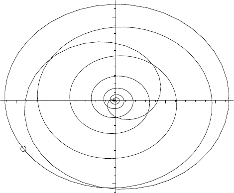
(c) Plot Bertie’s path for the complete circuit and superimpose an animation
of his motion on this path, representing Bertie as a moving circle.
After clearing Maple’s memory with the restart command,
>
restart:
Bertie’s radial and angular coordinates are entered.
>
r:=a*tˆ2*exp(-b*t)/(1+tˆ2); theta:=b+c*tˆ(2/3);
r :=
at
2
e
(−bt)
1+t
2
θ := b + ct
(2/3)
1
In 1872, the British writer Samuel Butler described a fictitious land in the utopian novel
Erewhon, the title being intended as an anagram for nowhere. In this land, the people dealt
with disease as a crime and destroyed machinery lest machines destroyed them. This would
not be the land for using computer algebra, so in the Computer Algebra Recipes series, I have
introduced a fictitious planet, Erehwon, where names are occasionally spelled backwards,
butErehwon is not backward in embracing modern technology.

8 INTRODUCTION
Note that entering theta for the angular coordinate has produced the Greek
symbol θ in the output.
Next, Bertie’s Cartesian coordinates, X = r cos θ, Y = r sin θ,arecalcu-
lated, the forms of r and θ being automatically substituted in the output.
>
X:=r*cos(theta); Y:=r*sin(theta);
X :=
at
2
e
(−bt)
cos(b + ct
(2/3)
)
1+t
2
Y :=
at
2
e
(−bt)
sin(b + ct
(2/3)
)
1+t
2
The speed V at time t is obtained by calculating V =
(dX/dt)
2
+(dY /dt)
2
.
>
V:=sqrt(diff(X,t)ˆ2+diff(Y,t)ˆ2);
V := ((
2 ate
(−bt)
cos(b + ct
(2/3)
)
1+t
2
−
at
2
be
(−bt)
cos(b + ct
(2/3)
)
1+t
2
−
2 at
3
e
(−bt)
cos(b + ct
(2/3)
)
(1 + t
2
)
2
−
2
3
at
(5/3)
e
(−bt)
sin(b + ct
(2/3)
) c
1+t
2
)
2
+(
2 ate
(−bt)
sin(b + ct
(2/3)
)
1+t
2
−
at
2
be
(−bt)
sin(b + ct
(2/3)
)
1+t
2
−
2 at
3
e
(−bt)
sin(b + ct
(2/3)
)
(1 + t
2
)
2
+
2
3
at
(5/3)
e
(−bt)
cos(b + ct
(2/3)
) c
1+t
2
)
2
)
(1/2)
The output looks quite messy, so let’s simplify it, making use of the simplify
command. One of the major difficulties with simplify is that the output may
not be simplified as much as you would like or not put into a specific form
that you are trying to attain. The simplify command comes with various
optional arguments, e.g., simplify(V,symbolic) as in the following command
line, which simplifies V assuming that all the parameters are positive.
>
V:=simplify(V,symbolic);
V :=
1
3
ate
(−bt)
(36 − 36 bt− 36 t
3
b +9t
2
b
2
+18t
4
b
2
+9t
6
b
2
+4t
(16/3)
c
2
+8t
(10/3)
c
2
+4t
(4/3)
c
2
)
(1/2)
(1 + t
2
)
2
This last result is certainly simpler than the previous one, all trig terms being
eliminated. Whether it’s the simplest possible form is a matter of taste. Sim-
plifying with Maple is usually a matter of trial and error and you will see many,
many simplification examples as you progress through this book.
To determine the distance d that Bertie flies over a time interval t =0 to
some arbitrary time T , an attempt is made to analytically evaluate the integral
d=
T
0
Vdtusing the integration (int) command.
>
d:=int(V,t=0..T);
d :=
T
0
1
3
ate
(−bt)
(36 − 36 bt− 36 t
3
b +9t
2
b
2
+18t
4
b
2
+9t
6
b
2
+4t
(16/3)
c
2
+8t
(10/3)
c
2
+4t
(4/3)
c
2
)
(1/2)
(1 + t
2
)
2
dt
INTRODUCTORY RECIPES 9
Maple is unable to find an analytic solution, returning the integral without
evaluating it. So, let’s enter the given parameter values, a =3, b = π/8, and
c = 10. Note that the command Pi for entering π is capitalized. Maple is case
sensitive here.
>
a:=3: b:=Pi/8: c:=10:
The time T =12.99 minutes, which is now entered, is the approximate time for
Bertie to complete one circuit. It is determined by trial and error by numerically
calculating the total distance to 4 digits, using the floating point evaluation
(evalf) command. Increasing T will not change the answer to this accuracy.
>
T:=12.99; distance:=evalf(d,4);
T := 12.99 distance := 23.98
Bertie travels a total distance of about 24 sretem in one complete circuit.
To animate Bertie’s flight and superimpose the motion on a plot of the entire
route, special plots commands are required. These are contained in the plots
library package, which is now “loaded”.
>
with(plots);
Warning, the name changecoords has been redefined
[animate, animate3d, ... display, ... polarplot, ... textplot3d, tubeplot]
The with( ) command is used to load Maple library packages. Normally, I
would place a colon on the above command line to suppress the output, but
here a partial list of the large number of specialized plot commands that are
available in the plots package is shown. The commands animate, polarplot (to
plot the trajectory in polar coordinates), and display (to superimpose graphs)
in the output list will be used here. There is also a warning message that the
name changecoords has been redefined. This warning appears even if a colon
is used. If desired, warnings can be removed by using a colon and inserting
the command interface(warnlevel=0) prior to loading the library package.
From now one, I will generally artificially remove all such warnings in the text.
In the first graph, gr1, an animation of Bertie’s motion is created with
the animate command. To fit into the width of the page, the lengthy Maple
command line is broken over two text lines. Bertie’s X and Y coordinates are
entered as a Maple list. The time range is taken from t =0toT . I have chosen
to use 500 frames (the default is 25) to make a reasonably smooth animation.
A point style is chosen, Bertie being represented by a size 16 blue circle. A
line-ending colon is used to prevent the plotting numbers from being displayed.
>
gr1:=animate([X,Y],t=0..T,frames=500,style=point,
symbol=circle,color=blue,symbolsize=16):
The polarplot command is used in gr2 to graph the entire route as a thick
(the default thickness is 0) orange line. To obtain a smooth curve, a minimum
of 500 (the default is 50) plotting points is requested.
>
gr2:=polarplot([r,theta,t=0..T],numpoints=500,style=line,
color=orange,thickness=2):
The graphs are now superimposed with the display command, the axis labels
10 INTRODUCTION
x and y being added. The double quotes denote that each enclosed item is a
“Maple string”. A string is a sequence of characters that has no value other
than itself. It cannot be assigned to, and will always evaluate to itself.
>
display([gr1,gr2],labels=["x","y"]);
–1
1
y
–1 1
x
Figure 3: Bertie’s patrol route while on sentry duty.
Figure 3 shows the entire path traced out by Bertie and his position (repre-
sented by the small circle) two minutes after he starts on his patrol route. The
animation can be initiated (the circle starts at the origin and moves along the
path, stopping when t = T =12.99 minutes.) by clicking on the computer plot
and then on the start arrow in the Maple tool bar at the top of the computer
screen. The animation may be made to repeat by clicking on the looped arrow
and stopped by clicking on the solid square. Other options are also available.
E.HowtoUsethisText
Although some of Maple’s basic syntax has been provided in these introduc-
tory recipes, it is recommended that the computer algebra novice start at the
beginning of the Appetizers, even if your mathematical physics background is
above that of the recipes presented there. It is in these early chapters that more
of the basic features of the Maple system are introduced. Further, you might be
surprised at how even initially simple problems can be made more interesting
and often much more challenging because of the fact that a computer algebra
system is being used. Whatever approach you adopt to using this book, I hope
that you savor the wide variety of mathematical physics recipes that follow.
Bon Appetit! Your computer algebra chef, Richard.
Part I
THE APPETIZERS
The last thing one discovers in composing a work
is what to put first.
Blaise Pascal, French scientist, philosopher (1623–62)
Each problem that I solved became a rule
which served afterwards to solve other problems.
Ren´e Descartes, French philosopher and mathematician (1596–1650)
Food probably has a very great influence on the
condition of men....Who knows if a well-prepared soup
was not responsible for the pneumatic pump
or a poor one for a war?
G. C. Lichtenberg, German physicist, philosopher (1742–99)

Chapter 1
Linear ODEs of Physics
In this chapter, the recipes illustrate how Maple may be used to solve and
explore some representative ordinary differential equations (ODEs) from the
world of physics. The focus is on linear ODEs (LODEs), i.e., those which
are first order or linear in the dependent variable. Although an example of a
nonlinear ODE (NLODE), i.e., one which contains one or more terms which
are not linear in the dependent variable, is presented in the second recipe, the
study of NLODEs is a much more mathematically challenging topic and will be
postponed until the Desserts.
This chapter is not intended to teach you all the details of the wide variety
of approaches for solving ODEs, but rather to show you how Maple can be used
as an auxiliary tool to implement some of the more common methods. However,
the series approach to solving an ODE will be postponed until Chapter 2.
As you are probably aware, the subject of solving differential equations (or-
dinary and partial) is huge. This is exemplified by Daniel Zwillinger’s Handbook
of Differential Equations [Zwi89] which is 700 pages long. This reference book
is highly recommended for quickly looking up every known method of solution.
1.1 Linear ODEs with Constant Coefficients
Consider an nth order LODE of the general structure (the spatial coordinate x
being replaced by t for time-dependent problems),
d
n
y
dx
n
+ a
n−1
(x)
d
n−1
y
dx
n−1
+ ···+ a
1
(x)
dy
dx
+ a
0
(x) y = f(x). (1.1)
If f(x) = 0, the ODE is said to be homogeneous, otherwise it is nonhomogeneous.
The first ODEs that physics and engineering students usually encounter are
differential equations with constant coefficients (a
0
, etc., independent of x)
which can be solved in closed form in terms of “elementary” (trigonometric,
logarithmic, exponential) functions using a variety of standard methods. In this
section, I will illustrate how Maple can be used to implement these methods,
bypassing the tedious intermediate steps involved in a hand calculation.

14 CHAPTER 1. LINEAR ODES OF PHYSICS
1.1.1 Dazzling Dsolve Debuts
One should never make one’s debut with a scandal.
One should reserve that to give an interest to one’s old age.
Oscar Wilde, Anglo-Irish playwright, author, The Picture of Dorian Gray (1891)
Whether the coefficients are constant or not, the dsolve command is dazzling
in its ability to solve LODEs. Before we tackle some physical examples, this
mathematical recipe briefly looks at what is possible with dsolve.
>
restart:
Let’s begin with the general nonhomogeneous first order LODE given in ode1 .
>
ode1:=diff(y(x),x)+a(x)*y(x)=f(x);
ode1 := (
d
dx
y(x)) + a(x) y(x)=f (x)
A standard method for solving ode1 is to first find its integrating factor, IF .
Loading the necessary DEtools package, the intfactor command yields IF .
>
with(DEtools): IF:=intfactor(ode1);
IF := e
(
a(x) dx)
The integral in IF is performed by specifying a(x), e.g., a(x)=a, a constant,
and applying the value command to IF.
>
a(x):=a: IF:=value(IF);
IF := e
(ax)
Multiplying ode1 by IF ,thefirst integral I1 is obtained by applying firint.
>
I1:=firint(IF*ode1);
I1 := e
(ax)
y(x) −
e
(ax)
f (x) dx + C1 =0
Since the ODE is first order, one arbitrary coefficient
C1 appears. To evaluate
the integral in I1 , f(x) must be given. Suppose, e.g., that f(x)=e
−x
.Forming
value(I1), the first integral is explicitly evaluated.
>
f(x):=exp(-x): I1:=value(I1);
I1 := e
(ax)
y(x) −
e
(ax−x)
a − 1
+
C1 =0
The general solution to ode1 , labeled y1 , follows on solving I1 for y(x).
>
y1:=solve(I1,y(x));
y1 := −
−e
(ax−x)
+ C1 a − C1
e
(ax)
(a − 1)
The above approach has mimicked the major steps of a hand calculation. The
same basic result can be obtained more quickly by applying dsolve to ode1 .
>
dsolve(ode1,y(x));
y(x)=(
e
(x (a−1))
a − 1
+
C1 ) e
(−ax)

1.1. LINEAR ODES WITH CONSTANT COEFFICIENTS 15
A common ODE notation is to use primes, each prime (
) standing for d/dx.
If desired, this notation can be introduced into the ODE output by first loading
the PDEtools library package and entering the following declare command.
>
with(PDEtools): declare(y(x),prime=x);
y(x) will now be displayed as y, derivatives with respect to x of functions
of one variable will now be displayed with
Then entering, say, the nonhomogeneous second-order linear ODE ode2 with
constant coefficients, produces an output with the prime notation.
>
ode2:=diff(y(x),x,x)+a1*diff(y(x),x)+a0*y(x)=F(x);
ode2 := y
+ a1 y
+ a0 y = F(x)
AnODEsuchasode2 can be classified by applying the odeadvisor command.
>
odeadvisor(ode2);
[[
2nd order , linear, nonhomogeneous]]
An even more important diagnostic tool is the infolevel[dsolve] command,
which will give information on what methods are used in attempting to solve the
ODE when dsolve is applied, even if unsuccessful. An integer between 1 and
5 must be specified, with generally more detailed information being provided
as the number is increased. On applying the dsolve command to ode2 ,the
method of attack is summarized in the following output and, in this case, the
general solution y(x) given with two arbitrary coefficients
C1 and C2 .
>
infolevel[dsolve]:=5: dsolve(ode2,y(x));
Methods for second order ODEs:
— Trying classification methods —
trying a quadrature
trying high order exact linear fully integrable
trying differential order: 2; linear nonhomogeneous with symmetry [0,1]
trying a double symmetry of the form [xi=0, eta=F(x)]
Try solving first the homogeneous part of the ODE
−> Tackling the linear ODE “as given”:
checking if the LODE has constant coefficients
<− constant coefficients successful
<− successful solving of the linear ODE ”as given”
−> Determining now a particular solution to the nonhomogeneous ODE
building a particular solution using variation of parameters
particular solution has integrals (!)
−> trying a d’Alembertian particular solution free of integrals
<− no simpler d’Alembertian solution was found
<− solving first the homogeneous part of the ODE successful

16 CHAPTER 1. LINEAR ODES OF PHYSICS
y = e
((−
a1
2
+
√
a1
2
−4 a0
2
) x)
C2 + e
((−
a1
2
−
√
a1
2
−4 a0
2
) x)
C1
+
e
(−
(−a1 +
√
a1
2
−4 a0 ) x
2
)
F (x) dx e
(x
√
a1
2
−4 a0 )
−
F (x) e
(
(a1 +
√
a1
2
−4 a0 ) x
2
)
dx
e
(−
(a1 +
√
a1
2
−4 a0 ) x
2
)
a1
2
− 4 a0
The corresponding homogeneous ODE (set F (x)=0) was first solved and then
a particular solution obtained for F (x) = 0 using the variation of parameters
method. The homogeneous solution is obtained by assuming that y ∼ e
λx
.This
yields λ
2
+a1 λ +a0 =0, which has two roots λ
1
and λ
2
. So the general solution
of the homogeneous ODE is of the form
C1 e
λ
1
x
+ C2 e
λ
2
x
, the specific forms
of λ
1
and λ
2
being easily identified from the above Maple output. The variation
of parameters method then assumes that y(x)=
C1(x) e
λ
1
x
+ C2(x) e
λ
2
x
for
the complete LODE, and solves for the functions
C1(x)and C2(x). See, for
example, [Ste87] for the details.
The infolevel[dsolve] command can be turned off by setting it to 0. The
prime notation can also be turned off by entering the command OFF.
>
infolevel[dsolve]:=0: OFF:
Boundary value and initial value problems are important in engineering and
physics. As a simple example of the former, suppose, e.g., that a1=2, a0=3,
and F (x)=x +sin(x) e
−x
.Thenode2 reduces to the form given in ode3 .
>
a1:=2: a0:=3: F(x):=x+sin(x)*exp(-x): ode3:=ode2;
ode3 := (
d
2
dx
2
y(x)) + 2 (
d
dx
y(x)) + 3 y(x)=x +sin(x) e
(−x)
Suppose that the boundary conditions (bcs) are that y(0) = y(1) = 0. The
boundary value problem is solved for y(x) by entering the equation name and
bcs in the dsolve command as a “Maple set” (items enclosed in braces, {}).
Unlike a list, a set does not preserve order or repetition.
>
dsolve({ode3,y(0)=0,y(1)=0},y(x));
y(x)=−
1
9
e
(−x)
sin(
√
2 x) (2 cos(
√
2) + e + 9 sin(1))
sin(
√
2)
+
2
9
e
(−x)
cos(
√
2 x)
+
1
9
e
(−x)
(3 xe
x
− 2 e
x
+9sin(x))
Now, an initial value problem is considered. First, let’s turn the declare
command back on and replace x with the time variable t in ode3 .
>
ON: ode4:=subs(x=t,ode3);
ode4 := y
t, t
+2y
t
+3y(t)=t +sin(t) e
(−t)
Because the independent variable is no longer x, the output has used the no-
tation y
t
and y
t, t
to indicate 1st and 2nd time derivatives. Now, suppose that