Enns R.H. Computer Algebra Recipes for Mathematical Physics

Подождите немного. Документ загружается.

1.1. LINEAR ODES WITH CONSTANT COEFFICIENTS 17

y(0) = 100 and y

(0) = 10. ode4 is now solved for y(t), subject to the initial

conditions. The diﬀerential operator D is used to enter the derivative condition.

dsolve({ode4,y(0)=100,D(y)(0)=10},y(t));

y(t)=

490

(−t)

sin(

√

2 t)

√

902

(−t)

cos(

√

2 t)+

(−t)

(3 te

− 2 e

+9sin(t))

To simplify y(t), the last output (indicated by %)mustﬁrstbeassigned. If

this is not done, entering y(t) would generate the output y(t), not the above

answer. Then y(t) is (somewhat) simpliﬁed and assigned the name y4 .

assign(%): y4:=simplify(y(t));

y4 :=

(−t)

(490 sin(

√

2 t)

√

2 + 902 cos(

√

2 t)+3te

− 2 e

+9sin(t))

ODE systems may also be solved with the dsolve command. Consider the

coupled ﬁrst-order time-dependent LODEs given in ode5a and ode5b.

ode5a:=diff(x(t),t)=-3*x(t)+4*z(t)+(sin(t))ˆ2*exp(-2*t);

ode5a := x

= −3 x (t)+4z (t)+sin(t)

(−2 t)

ode5b:=diff(z(t),t)=2*z(t)-5*x(t)+(cos(t))ˆ3;

ode5b := z

=2z (t) − 5 x(t) + cos(t)

The set of ODEs, ode5a and ode5b, is solved for the set of unknown functions,

x(t)andz(t), subject to the initial conditions x(0)=100 and z(0)= 10.

sol:=dsolve({ode5a,ode5b,x(0)=100,z(0)=10},{x(t),z(t)});

The solution sol, whose lengthy output has been suppressed here in the text,

is assigned, and exponential terms collected in x(t)andz(t), the results being

labeled X and Z, respectively.

assign(sol): X:=collect(x(t),exp); Z:=collect(z(t),exp);

X:= (−

57231

7480

sin(

√

55 t

)

√

55 +

203147

2040

cos(

√

55 t

)) e

(−

)

cos(2 t) −

) e

(−2 t)

170

cos(t)+

170

sin(t)+

sin(3 t)+

cos(3 t)

Z := (

15727

1632

cos(

√

55 t

) −

90973

5280

sin(

√

55 t

)

√

55) e

(−

)

−

sin(t)

cos(t)+

cos(3 t) −

sin(3 t)+(−

sin(2 t)+

cos(2 t) −

) e

(−2 t)

If you are not already dazzled by the power of dsolve in obtaining the above

result try, e.g., some other nonhomogeneous terms in the ODEs. Unlike with

the hand calculation, a new answer can be rapidly and accurately generated.

To this point, we have had no control over the method of solution. As shall

be demonstrated in some of the following recipes, various self-evident options

can be included in dsolve,suchasseries, laplace, numeric, etc.

18 CHAPTER 1. LINEAR ODES OF PHYSICS

1.1.2 The Tale of the Turbulent Tail

Nonsense. Space is blue and birds ﬂy through it.

Felix Bloch, 1952 Nobel laureate in physics, Heisenberg and the early days of

quantum mechanics, Physics Today, December 1976

As a post-doctoral fellow at the Chadwick Laboratory at the University of

Liverpool (England), I enjoyed my leisure time on dark, rainy, often foggy,

winter nights playing badminton with my fellow physicists. The Tale of the

Turbulent Tail is inspired by those games of badminton played so long ago.

In an article contained in a delightful reprint collection entitled The Physics

of Sports [PLA92], Peastrel, Lynch and Armenti reported on their experimental

investigation of the aerodynamics of a badminton shuttlecock or “bird” falling

vertically from rest. The relevant data is reproduced in Table 1.1, the distance

y in meters that the bird fell in t seconds being given.

Table 1.1: Data for the falling badminton bird.

t 0.347 0.470 0.519 0.582 0.650 0.674 0.717 0.766

y 0.61 1.00 1.22 1.52 1.83 2.00 2.13 2.44

t 0.823 0.870 1.031 1.193 1.354 1.501 1.726 1.873

y 2.74 3.00 4.00 5.00 6.00 7.00 8.50 9.50

From the last pair of entries in the table, Peastrel et al calculated the terminal

velocity (occuring when the downward gravitational force balances the upward

drag force due to air resistance) to be (9.50 −8.50)/(1.873 −1.726) = 6.8 m/s.

The gravitational acceleration was taken to be g =9.8m/s

The investigators’ goal was to determine which law of air resistance could

best account for the experimental data, Stokes’s law or Newton’s law. For the

Stokes model, the drag force on a body of mass m moving with velocity v is

given by F

Stokes

= −amv, while for the Newton model, F

Newton

= −bm|v|v.

The positive coeﬃcients a and b can be related to the terminal velocity and g.

After loading the plots library package, I will begin this recipe by ﬁrst

restart: with(plots):

entering the experimental data of Table 1.1 so that the predictions of the two

models can be tested for goodness of ﬁt. The data is entered as a “list of lists.”

The ﬁrst entry in each list is the time, the second entry the distance.

data:=[[0.347,0.61],[0.470,1.00],[0.519,1.22],[0.582,1.52],

[0.650,1.83],[0.674,2.00],[0.717,2.13],[0.766,2.44],

[0.823,2.74],[0.870,3.00],[1.031,4.00],[1.193,5.00],

[1.354,6.00],[1.501,7.00],[1.726,8.50],[1.873,9.50]]:

Taking the gravitational force on the bird to be mg and assuming that Stokes’s

law of air resistance prevails (a comment (preﬁxed by the sharp symbol #)to

this eﬀect is added to the end of the command line), the acceleration of the

bird is given by ode1 . This is a ﬁrst-order linear nonhomogeneous ODE.

1.1. LINEAR ODES WITH CONSTANT COEFFICIENTS 19

ode1:=diff(v(t),t)=g-a*v(t); #Stokes’s resistance law

ode1 :=

v(t)=g − av(t)

After a suﬃciently long time, the gravitational and drag forces will balance and

the bird will reach its terminal velocity V1 = g/a. So the unknown constant a

can be eliminated by substituting a = g/V1 into ode1 .

ode1:=subs(a=g/V1,ode1);

ode1 :=

v(t)=g −

gv(t)

Since the bird falls from rest, the initial value problem is solved by entering

ode1 and the initial condition v(0) =0 in the dsolve command as a Maple set.

sol1:=dsolve({ode1,v(0)=0},v(t));

sol1 := v(t)=V1 − e

(−

)

To compare with the experimental data, we need to calculate the distance that

the bird falls in T seconds. For the Stokes model, this distance y1 is obtained

by integrating the right-hand side (rhs) of sol1 from t =0toT .

y1:=int(rhs(sol1),t=0..T);

y1 :=

V1 (−V1 + gT + V1 e

(−

)

Let’s now look at Newton’s model of air resistance. Since the motion is

in one direction (down) only, the absolute value sign can be dropped, so that

Newton

= −bmv

. The acceleration of the bird is now given by ode2 .Thisis

a ﬁrst order nonlinear nonhomogeneous ODE.

ode2:=diff(v(t),t)=g-b*v(t)ˆ2; #Newton’s resistance law

ode2 :=

v(t)=g − bv(t)

The terminal velocity is now given by V2 =



g/b. The unknown constant b is

removed from the equation by substituting b = g/V2

into ode2 .

ode2:=subs(b=g/V2ˆ2,ode2);

ode2 :=

v(t)=g −

gv(t)

To see what methods are used in trying to solve ode2 ,theinfolevel[dsolve]

command is entered and set to 2. Applying the dsolve command to ode2 and

taking the rhs, an analytic solution v2 is generated for the velocity v(t).

infolevel[dsolve]:=2: v2:=rhs(dsolve(ode2,v(t)));

Methods for ﬁrst order ODEs:

— Trying classiﬁcation methods —

trying a quadrature

trying 1st order linear

trying Bernoulli

trying separable

20 CHAPTER 1. LINEAR ODES OF PHYSICS

<− separable successful

v2 :=

2 V2 e

(

2 tg

2 C1 g

)

1+e

(

2 tg

2 C1 g

)

− V2

Maple has used the fact that ode2 is separable. A separable ([Ste87]) ﬁrst-order

nonlinear ODE can be written in the form dy/dx = g(x) f(y). It is solved by

separating variables and integrating, i.e.,



dy/f(y)=



g(x) dx.

The arbitrary constant

C1 is determined by evaluating v2 at t= 0, setting

the result to 0, and solving for

C1. On some executions, C1 involves I ≡

√

−1,

so to ensure a real velocity v2 , the complex evaluation command (evalc breaks

a complex quantity into real and imaginary parts) is applied to v2 .

_C1:=solve(eval(v2,t=0)=0,_C1); v2:=evalc(v2);

C1 := 0 v2 :=

2 V2 e

(

2 tg

)

1+e

(

2 tg

)

− V2

The distance y2 that the bird falls in T seconds, according to Newton’s model,

is now calculated by integrating v2 assuming that g>0, V2 > 0, and T>0.

y2:=int(v2,t=0..T) assuming g>0,V2>0,T>0;

y2 :=

V2 (V2 ln(1 + e

(

2 Tg

)

) − gT − V2 ln(2))

So, which is the better model equation, y1 or y2 ? Entering the values of g, V1,

and V2 , the forms of y1 and y2 arethenasfollows:

g:=9.8: V1:=6.8: V2:=6.8: y1:=y1; y2:=evalf(y2);

y1 := −4.718367347 + 6.800000000 T +4.718367347 e

(−1.441176471 T )

y2 := −3.270523024 + 4.718367347 ln(1. + e

(2.882352940 T )

) − 6.800000000 T

The experimental data is now plotted in gr1, the data points being represented

by size 14 (red by default) circles.

gr1:=plot(data,style=point,symbol=circle,symbolsize=14):

The theoretical curves y1 and y2 are plotted in gr2 overthetimeintervalT =0

to 2 seconds. y1 is represented by a thick blue dashed line, y2 by a thick green

solid line. The entry linestyle=[3,1] would produce the same line styles.

gr2:=plot([y1,y2],T=0..2,color=[blue,green],

linestyle=[DASH,SOLID],thickness=2):

The two graphs are then superimposed with the display command. The min-

imum number of tickmarks along the horizontal and vertical axes is speciﬁed,

and axis labels and a title added.

display({gr1,gr2},tickmarks=[4,3],labels=["t","y"],title=

"Newton’s law (solid green), Stokes’s law (dashed blue)");

The resulting picture is shown in Figure 1.1. It is clear that Newton’s law of

resistance is the correct model for the falling badminton bird. Stokes’s law is

1.1. LINEAR ODES WITH CONSTANT COEFFICIENTS 21

Newton’s law (solid line), Stokes’s law (dashed line)

Figure 1.1: The experimental points agree with Newton’s resistance law.

known to apply to the laminar ﬂow of air about a smooth moving object, while

Newton’s law applies to the turbulent ﬂow around a non-smooth body. It is the

tail “feathers” of the moving badminton bird which create the turbulence.

1.1.3 This Bar Doesn’t Serve Drinks

By the time a bartender knows what drink a man will have

before he orders, there is little else about him worth knowing.

Don Marquis, American humorist and journalist, (1878–1937)

This recipe involves a bar undergoing rotational motion. No, I don’t mean

that the local pub appears to be spinning because one has overindulged in liq-

uid refreshments after a tough exam! It has to do with the possible deﬂection

modes ([Mor48], [Hil57], [SR66]) of an originally straight uniform solid bar of

length L which rotates in a horizontal plane about one end (say x =0) with

uniform angular velocity ω. Below a critical frequency ω

, the bar remains

straight, but on exceeding ω

it starts pulsating and its shape changes. On fur-

ther increasing ω, another critical value ω

is reached, above which the shape

changes again, and so on. The values of the critical frequencies and the de-

ﬂection modes depend on how the ends of the bar are supported. Here, I will

consider one possibility, leaving it to you to explore other boundary conditions.

For small deﬂections y(x) from the straight shape, the governing 4th order

LODE (each prime denoting an x derivative) is



− k

y =0, where k

≡ω

/(YI). (1.2)

Here  is the mass per unit length, Y is Young’s modulus, and I is the moment

of inertia of a cross-section of the shaft about an axis perpendicular to the

xy plane. To solve the boundary value problem, four boundary conditions are

required for the homogeneous fourth-order equation, two conditions for each

22 CHAPTER 1. LINEAR ODES OF PHYSICS

end of the bar. I will consider the case when the pivot point at x =0 is a

clamped end (both y and the slope y



vanish at x =0), while x=L is a free end

(both y



(∝ bending moment) and y



(∝ shearing force) vanish at x= L).

The recipe begins with the loading of the plots library package and the

entry of the infolevel[dsolve] command. The PDE tools library is also

accessed and the declare command used to generate the prime notation.

restart: with(plots): infolevel[dsolve]:=2:

with(PDEtools): declare(y(x),prime=x);

The governing ODE (1.2) is entered. Instead of inputting the fourth derivative

as diff(y(x),x,x,x,x), the short-cut entry diff(y(x),x$4) is used.

ode:=diff(y(x),x$4)-kˆ4*y(x)=0;

ode := y



− k

y =0

The general solution of ode is obtained using the dsolve command and the

rhs of the result taken. Maple recognizes that ode is a LODE with constant

coeﬃcients and makes use of this fact to solve the equation.

y:=rhs(dsolve(ode,y(x)));

Methods for high order ODEs:

— Trying classiﬁcation methods —

trying a quadrature

checking if the LODE has constant coeﬃcients

<− constant coeﬃcients successful

y :=

C1 e

(−kx)

+ C2 e

(kx)

+ C3 sin(kx)+ C4 cos(kx)

Clamped-end boundary conditions are applied at x =0 in bc1 and bc2 ,and

free-end boundary conditions at x=L in bc3 and bc4 .

bc1:=eval(y,x=0)=0; bc2:=eval(diff(y,x),x=0)=0;

bc1 :=

C1 + C2 + C4 =0

bc2 := −

C1 k + C2 k + C3 k =0

bc3:=eval(diff(y,x$2),x=L)=0; bc4:=eval(diff(y,x$3),x=L)=0;

bc3 :=

C1 k

(−kL)

+ C2 k

(kL)

− C3 sin(kL) k

− C4 cos(kL) k

bc4 := −

C1 k

(−kL)

+ C2 k

(kL)

− C3 cos(kL) k

+ C4 sin(kL) k

Applying the analytic solve command, the set of four boundary conditions are

solved for the set of four unknown coeﬃcients. All the coeﬃcients are zero,

which corresponds to the trivial solution y(x)= 0, i.e., the straight bar proﬁle.

solve({bc1,bc2,bc3,bc4},{_C1,_C2,_C3,_C4});

{

C1 =0, C4 =0, C3 =0, C2 =0}

To obtain a non-trivial result, let’s ﬁrst solve the set of three boundary condi-

tions, bc1 , bc2 ,andbc4 ,for

C1, C2, and C4 and assign the solution sol.

sol:=solve({bc1,bc2,bc4},{_C1,_C2,_C4}); assign(sol):

C1, C2, and C4 are automatically substituted into the remaining boundary

condition, bc3 , which is divided by k

and simpliﬁed.

1.1. LINEAR ODES WITH CONSTANT COEFFICIENTS 23

bc3:=simplify(bc3/kˆ2);

bc3 := −

C3 (e

(−kL)

cos(kL)+2+e

(kL)

cos(kL))

(−kL)

− e

(kL)

+2sin(kL)

For a non-trivial solution,

C3 = 0, so the term containing cos(kL)mustbe

zero. The select command is used to extract this term from the lhs of bc3 .

eq:=select(has,lhs(bc3),cos(k*L))=0;

eq := e

(−kL)

cos(kL)+2+e

(kL)

cos(kL)=0

The expression eq is converted completely to trigonometric form and simpliﬁed.

eq2:=simplify(convert(eq,trig)/2);

eq2 := cos(kL)cosh(kL)+1=0

eq2 is a transcendental equation which must be solved numerically for kL.The

algebraic substitution kL= K is now made in eq2 .

eq3:=algsubs(k*L=K,eq2);

eq3 := cos(K)cosh(K)+1=0

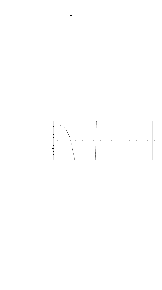
The lhs of eq3 is plotted in Figure 1.2, the viewing range being controlled.

plot(lhs(eq3),K=0..12,thickness=2,view=[0..12,-5..5]);

–4

Figure 1.2: Graphically locating the zeros of the transcendental equation.

The approximate values of the zeros of eq3 can be determined by visual inspec-

tion. A slightly more accurate procedure is to place the cursor on the zero on

the computer screen and click the mouse. The horizontal and vertical coordi-

nates of the cursor location are displayed in a small viewing box at the top left

of the computer screen. Numerical values of the zeros to 10 digits accuracy can

be obtained by applying the numerical solving command,

fsolve,toeq3 .If

lesser accuracy is desired, e.g., 5 digits, the Digits command can be used.

Digits:=5:

A “functional”, or “arrow” operator

f is introduced to systematically search

for the K zeros in the range 3 (n−1) to 3 n using the fsolve command. Dividing

by L then yields the k zeros.

f:=n->fsolve(eq3,K,3*(n-1)..3*n)/L:

When a number n is supplied, then subsequently entering f(n) will yield the

zero (if one exists) in the given range. For n = 1 the search range is 0 to 3, for

This command implements Newton’s method. [Ste87]

Created on the keyboard with the hyphen (-) followed by the greater than symbol (>).

24 CHAPTER 1. LINEAR ODES OF PHYSICS

n= 2 the range is 3 to 6, and so on. The sequence command, seq, is used in sol2

to generate the ﬁrst four zeros of eq2 . Note that the k’s have been subscripted,

the input syntax being k[n]. The zeros are then assigned.

sol2:=seq(k[n]=f(n),n=1..4); assign(sol2):

sol2 := k

1.8751

4.6941

7.8548

10.996

The transcendental equation eq3 may be rewritten as cos(K)=−1/ cosh(K).

For large K,cosh(K) →∞, so cos(K) → 0andk

→ (m − 1/2) π/L for large

integer m. Setting a ≡



YI/, the ﬁrst four critical frequencies are calculated.

critical_freq:=seq(omega[n]=a*k[n]ˆ2,n=1..4);

critical freq := ω

3.5160 a

,ω

22.035 a

,ω

61.698 a

,ω

120.91 a

The coeﬃcient C3 is collected in y, the result evaluated at k = k

, and the

sequence command used to generate the proﬁles Y

of the ﬁrst four deﬂection

modes. For brevity, only Y

is shown here in the output of sol3 .

sol3:=seq(Y[n]=eval(collect(y,_C3),k=k[n]),n=1..4);

sol3 := Y

=(0.18111 e

(

1.8751 x

)

+1.1811 e

(−

1.8751 x

)

+sin(

1.8751 x

)

− 1.3622 cos(

1.8751 x

))

C3 ,

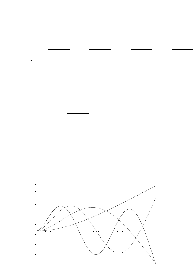
sol3 is assigned and the ﬁrst four possible deﬂection modes plotted for L =5

and

C3=1/5, the picture being shown in Figure 1.3. The solid curve with one

zero corresponds to n= 1, the dashed curve with two zeros to n=2, etc.

assign(sol3): L:=5: _C3:=1/5:

plot([seq(Y[n],n=1..4)],x=0..5,color=[red,green,blue,cyan],

linestyle=[SOLID,DASH,DOT,SOLID],labels=["x","y"]);

–0.4

–0.2

0.2

0.4

1234

Figure 1.3: First four deﬂection modes for the rotating bar.

1.1. LINEAR ODES WITH CONSTANT COEFFICIENTS 25

1.1.4 Shake, Rattle, and Roll

Principles aren’t of much account anyway, except at election time.

After that you hang them up to let them season.

Mark Twain, American author, Municipal Corruption, speech, 4 Jan. 1901

It is election time on the planet Erehwon and the politicians are traveling far

and wide to woo potential voters. Presidential candidate Amai Koorc is trav-

eling on his own personal three-coach train which rides along a guide-way on

a cushion of air. The middle coach (mass M>m) is occupied by Koorc and

other political “heavies”, while the outer two coaches (each of mass m) contain

media “light weights”. Each outer coach is connected to the middle one by an

identical linear spring (i.e, governed by Hooke’s law) with spring constant K.

All three coaches were initially sitting stationary on a straight stretch of the

guide-way with the coupling springs unstretched, when fringe members of the

opposition party imparted an impulse to each coach causing the train to start

“rolling” down the track in an erratic fashion which shook up the politicians

and rattled the media. This recipe simulates the motion of the train.

To simplify the ﬁnal results, it is assumed

that K, m,andM are positive.

restart: with(plots): assume(K>0,m>0,M>0):

Using Hooke’s law for the relative displacements x(t), y(t), and z(t)attimet

of the outer left, middle, and outer right coaches from equilibrium, Newton’s

second law yields the following three equations of motion.

ode1:=m*diff(x(t),t,t)=K*(y(t)-x(t));

ode1 := m (

x(t)) = K (y(t) − x (t))

ode2:=M*diff(y(t),t,t)=K*(z(t)-y(t))-K*(y(t)-x(t));

ode2 := M (

y(t)) = K (z (t) − y(t)) − K (y(t) − x(t))

ode3:=m*diff(z(t),t,t)=-K*(z(t)-y(t));

ode3 := m (

z(t)) = −K (z(t) − y(t))

This is a system of three coupled second-order LODEs with constant coeﬃcients.

Given the general initial condition (dots indicating time derivatives) x(0) = A,

y(0)= B, z(0) =C,˙x(0)=V 1, ˙y(0)= V 2, and ˙z(0) =V 3,

ic:=(x(0)=A,y(0)=B,z(0)=C,D(x)(0)=V1,D(y)(0)=V2,D(z)(0)=V3):

it would be very tedious to solve for x(t), y(t), and z(t) by hand. Even Maple

needs some guidance here as to what method is best to use. If no method

Note that assume applies the assumption throughout the entire worksheet, whereas

assuming applies it only in the command line that it is used. By default, assumed quan-

tities have attached “trailing tildes” in the output. The tildes can be removed by inserting

interface(showassumed=0) prior to the assumption. If desired, they can be removed from

all worksheets by clicking on File in the tool bar, then on Preferences, I/O Display, No

Annotation, and Apply Globally.

26 CHAPTER 1. LINEAR ODES OF PHYSICS

option is speciﬁed, applying the dsolve command to the three ODEs, sub-

ject to the initial condition, would yield a long “messy” result. Including the

method=laplace option, which makes use of the Laplace transform method,

yields a somewhat simpler, but still lengthy, answer (not shown here).

sol:=dsolve({ode1,ode2,ode3,ic},{x(t),y(t),z(t)},

method=laplace);

Using the list format [sin,cos], sine terms are now collected ﬁrst in sol,and

then cosine terms. Since the analytic expressions are still lengthy, only x(t)is

displayed here in the text.

sol2:=collect(sol,[sin,cos]);

sol2 := {x(t)=



(V1 − V3 )sin(



t)+(

−

) cos(



(

2 m + M

)

(3/2)



sin(



K (2 m + M)

t)(V3 − 2 V2 + V1 )

M (−2 B + C + A) cos(



K (2 m + M)

2 m + M

M (2 B +2t V2 )+2m (t V1 + C + A + t V3 )

2(2m + M)

, ······}

Recalling that x(t) represents the displacement of the ﬁrst outer coach from

equilibrium, it can be seen that the motion is built up of two parts. The trig

terms represent an oscillatory motion of the coach, while the last term corre-

sponds to a translational motion as time t increases. The oscillatory part is gov-

erned by two characteristic frequencies, ω =



K/m and



K (2 m + M)/(Mm).

The solution sol2 is now assigned and a functional operator f created to

substitute parameter values into each solution and simplify the result.

assign(sol2): f:=z->simplify(subs(par,z(t))):

The three coaches were initially in their equilibrium positions so A=B =C =0.

In some suitable set of Erehwonese units, the initial speeds imparted to the

coaches by the opposition gang were V 1=2/3, V 2=−1/3, and V 3=1/6.

Each coach containing light-weight media had a mass m =1 while the political

heavies’ coach had a mass M =2. The spring constant K =4.

par:=(A=0,B=0,C=0,V1=2/3,V2=-1/3,V3=1/6,m=1,M=2,K=4):

If the ﬁrst outer coach was initially located at X = 1, the middle one at Y =2,

and the other outer coach at Z =3, their positions at time t areasfollows.

X:=1+f(x); Y:=2+f(y); Z:=3+f(z);

The Laplace transform of x(t) is deﬁned as L(x(t)) ≡ X(s)=



∞

x(t)e

−st

dt. Integrating

by parts and assuming e

−st

x(t) → 0ast →∞,thenL(˙x)=sX(s) − x(0), and L(¨x)=

X(s)−sx(0)− ˙x(0). To solve a LODE with constant coeﬃcients, one can Laplace transform

the LODE, solve the resulting algebraic equation for X(s), and then perform the inverse

transform to obtain x(t). Laplace transforms are discussed in Chapter 6.