Enns R.H. Computer Algebra Recipes for Mathematical Physics

Подождите немного. Документ загружается.

1.2. LINEAR ODES WITH VARIABLE COEFFICIENTS 37

and the parameter L (short for λ), and Y for generating the general analytic

solution of a speciﬁed ode and taking the right-hand side of the result.

restart:

SL:=(p,q,w,L)->diff(p*diff(y(x),x),x)-q*y(x)+L*w*y(x)=0;

SL := (p, q, w, L) → (

(p (

y(x)))) −q y(x)+Lwy(x)=0

Y:=ode->rhs(dsolve(ode,y(x))):

According to standard texts (e.g., [MW71], [Boa83]), Bessel’s’ equation should

result on choosing p = x, q = −x, w = −1/x,andL ≡ λ = −n

. Entering these

speciﬁc forms as arguments in SL produces ode1 .

ode1:=SL(x,-x,1/x,-nˆ2);

ode1 := (

y(x)) + x (

y(x)) + x y(x) −

y(x)

Loading the DEtools library package, Jennifer enters the following odeadvisor

command line to see if Maple can classify ode1 and oﬀer any information about

this equation. The ODE is identiﬁed as Bessel’s equation and inclusion of the

help option causes a help page to be opened with information on this equation.

She adds a comment to close the help page when ﬁnished reading it.

with(DEtools): odeadvisor(ode1,help); #close Help page

[

Bessel]

Entering the infolevel[dsolve] command so as to gain information about

the methods tried in attempting to solve the ODE, she then uses the arrow

operator Y to solve ode1 .

infolevel[dsolve]:=2: y1:=Y(ode1);

Methods for second order ODEs:

— Trying classiﬁcation methods —

trying a quadrature

checking if the LODE has constant coeﬃcients

checking if the LODE is of Euler type

trying a symmetry of the form [xi=0, eta=F(x)]

checking if the LODE is missing ’y’

−> Trying a Liouvillian solution using Kovacic’s algorithm

<− No Liouvillian solutions exists

−> Trying a solution in terms of special functions:

−> Bessel

<− Bessel successful

<− special function solution successful

y1 :=

C1 BesselJ(n, x)+ C2 BesselY(n, x)

After identifying the ODE as second order, Maple tries various approaches be-

fore seeking and obtaining a general special function solution in terms of Bessel

functions. Highlighting, say, BesselJ in the output with the mouse and clicking

on “Help on BesselJ”, opens a help page on Bessel functions. BesselJ(n, x)is

38 CHAPTER 1. LINEAR ODES OF PHYSICS

identiﬁed as a Bessel function of the ﬁrst kind of order n, while BesselY(n, x)

is a Bessel function of the second kind. In standard mathematical notation,

they are usually written as J

(x)andY

(x), respectively. Before delving into

some of the properties of Bessel functions, Jennifer notes that on executing the

command ?inifcns, a help page is opened which lists all the functions known

to Maple and has hyperlinks to associated help pages (e.g., for BesselJ).

?inifcns;

Closing the help page, Jennifer forms an arrow operator f for plotting a se-

quence of four (the number can be easily changed) Bessel functions with integer

subscript. The name N (BesselJ or BesselY) of the Bessel function must be

supplied along with the horizontal range x = x1tox2 over which the function

is to be plotted. The four curves are given diﬀerent colors and line styles. Line

style 4 produces a DASH-DOT curve. The vertical range is limited with the

view command to −1to+1becausetheY

(x) become inﬁnitely large at x=0

if this point is included in the range of interest.

f:=(N,x1,x2)->plot([seq(N(n,x),n=0..3)],x=x1..x2,thickness=2,

color=[red,blue,green,cyan],linestyle=[1,2,3,4],

view=[x1..x2,-1..1],tickmarks=[2,2]):

Making use of f,theJ

(x)andY

(x) are plotted for x=x1=0 to x2=20.

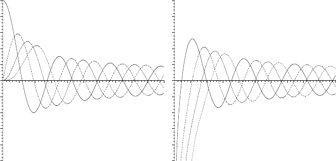
f(BesselJ,0,20); f(BesselY,0,20);

–1

10 20

–1

10 20

Figure 1.8: Left plot: Left to right, J

to J

.Right:Lefttoright,Y

to Y

The Bessel functions J

(x), J

(x), and J

(x) are ordered from left to

right in the left plot of Figure 1.8. At x=0, J

has the value 1, while all other

positive integer J

are equal to zero there. The Bessel functions Y

(x), Y

(x),

(x), and Y

(x), with the same ordering, are shown on the right of Figure 1.8.

The Y

(x) diverge to −∞ at x = 0, so are rejected in physical problems where

the origin is part of the range of interest.

1.2. LINEAR ODES WITH VARIABLE COEFFICIENTS 39

Of particular importance in solving problems involving Bessel functions is

knowing the locations of the zeros. The ﬁrst 5 zeros of, e.g., J

are now ob-

tained with the following BesselJZeros command. Note that the argument 1

is expressed in ﬂoating point form, i.e., 1.0, in order to numerically evaluate the

zeros. The command BesselYZeros will generate the zeros of the Y

(x).

Zeros_J1:=BesselJZeros(1.0,1..5);

Zeros

J1 := 3.831705970, 7.015586670, 10.17346814, 13.32369194, 16.47063005

For large x, both the J

(x)andY

(x) have the appearance of slowly decreasing

sine or cosine functions. Jennifer conﬁrms this conjecture by Taylor expanding,

e.g., J

(x)aboutx=+∞ and keeping the ﬁrst term in the expansion.

taylor(BesselJ(1,x),x=infinity,1);

−

√

2 cos(x +

)



√

+O((

)

(3/2)

)

The “order of” term, O((1/x)

3/2

), is removed with convert(%,polynom),the

“ditto operator”, %, applying the command to the previously executed result.

J1_asymptotic:=convert(%,polynom);

asymptotic := −

√

2 cos(x +

)



√

Asymptotically, J

(x) behaves like a cosine function whose amplitude decreases

like 1/

√

x. The Bessel functions have many important properties which are too

numerous for Jennifer to explore here. For an exhaustive list of the properties

of all special functions, she refers the reader to the voluminous Handbook of

Mathematical Functions [AS72]. One important property shared by special

functions is that they satisfy recurrence relations, relating functions of diﬀerent

orders. Here’s an example of a recurrence relation for the J

(x). This recurrence

relation relates Bessel functions of orders n−1, n+1, and n for arbitrary x.

recurrence:=BesselJ(n-1,x)+BesselJ(n+1,x)

=simplify(BesselJ(n-1,x)+BesselJ(n+1,x));

recurrence := BesselJ(n − 1,x) + BesselJ(n +1,x)=

2 n BesselJ(n, x)

Now, Jennifer introduces Legendre’s ODE by entering the Sturm–Liouville

arrow operator SL with p =1−x

, q =0, w =1, and L ≡ λ = n (n + 1). The

diﬀerential equation ode2 is then solved and identiﬁed as Legendre’s equation.

ode2:=SL(1-xˆ2,0,1,n*(n+1)); y2:=Y(ode2);

ode2 := −2 x (

y(x)) + (1 −x

)(

y(x)) + n (n +1)y(x)=0

Methods for second order ODEs:

...................................................................

To recall the second previous result, use two percent signs, %%, and so on.

40 CHAPTER 1. LINEAR ODES OF PHYSICS

−> Trying a solution in terms of special functions:

−> Bessel

−> elliptic

−> Legendre

<− Legendre successful

<− special function solution successful

y2 :=

C1 LegendreP(n, x)+ C2 LegendreQ(n, x)

Highlighting LegendreP with the mouse and opening up the associated help page

reveals that LegendreP(n, x)istheLegendre function of the ﬁrst kind of order n,

while LegendreQ(n, x)istheLegendre function of the second kind. In standard

mathematical notation, they are written as P

(x)andQ

(x), respectively. If

the odeadvisor command is applied to ode2 , the ODE is identiﬁed

odeadvisor(ode2);

[

Gegenbauer]

as a Gegenbauer equation, which has the general structure [AS72],

(1 − x

) y



− (2 α +1)xy



+ n (n +2α) y =0. (1.7)

Legendre’s ODE is a special case of Equation (1.7) with α=1/2.

The Legendre functions P

(x)withn = 0 or a positive integer play an im-

portant role in boundary value problems involving spherical polar coordinates,

in which case x = cos(θ)whereθ is the polar angle measured from the z-axis.

The polar angle runs from 0 to π radians, so x spans the range 1 to −1. For

n =0, 1, 2, ...,theP ’s reduce to the Legendre polynomials which Jennifer now

generates for n = 0 to 5. The simplify command must be applied to produce

the ﬁnite polynomial forms.

Ps:=seq(simplify(LegendreP(n,x)),n=0..5);

Ps := 1,x,−

3 x

−

The polynomials may also be generated by loading the orthopoly library package

and using the syntax P(n,x) to enter the nth order Legendre polynomial.

with(orthopoly): seq(P(n,x),n=0..5);

1,x,−

3 x

−

To produce Q

(x) over the range x=−1 to 1, Jennifer enters EnvLegendreCut:

=1..infinity: which selects the desired mathematical branch

of the function.

The Q ’s are then produced for n=0, 1, 2. They are expressible as combinations

of log functions.

_EnvLegendreCut:=1..infinity:

Qs:=seq(simplify(LegendreQ(n,x)),n=0..2);

To plot Q

(x)for|x| > 1, enter EnvLegendreCut:=-1..1: and adjust the view.

1.2. LINEAR ODES WITH VARIABLE COEFFICIENTS 41

Qs :=

ln(1 + x) −

ln(1 − x),

x ln(1 + x) −

x ln(1 − x) − 1,

−

ln(1 + x)+

ln(1 − x)+

ln(1 + x) −

ln(1 − x) −

3 x

Using the arrow operator f, the Legendre functions of both kinds are now

plotted for n=0 to 3 over the horizontal range x= −1to1.

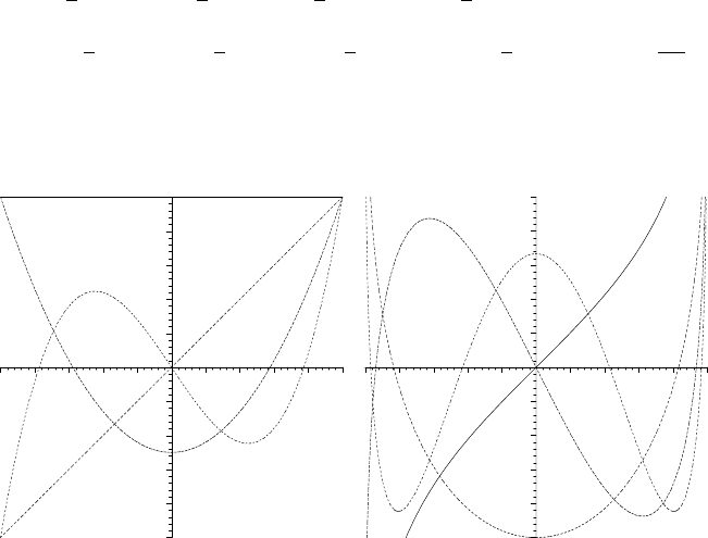
f(LegendreP,-1,1); f(LegendreQ,-1,1);

–1

–1 1

–1

–1 1

Figure 1.9: Left plot: P

, P

.Right:Q

, Q

(x) (horizontal curve), P

(x) (diagonal curve), P

(x) (parabola), and P

(x)

(N-shape) are shown in the left plot of Figure 1.9. Q

(x) (solid curve), Q

(x)

(parabola), Q

(x) (N-shape), and Q

(x) (W-shape) are shown in the right plot

of the ﬁgure. The P

are well behaved at x = ±1, but the Q

diverge at these

points and must be rejected in physical problems which include x = ±1inthe

range of interest.

An important general property that all solutions y

(x) of the Sturm–Liouville

equation corresponding to a given λ

possess is orthogonality. Provided that

y(x), or y



(x), or p(x) vanishes at the end points a and b of the range (referred

to as Sturm–Liouville boundary conditions), then



w(x) y

(x) y

(x) dx =0, for m = n. (1.8)

w(x)isreferredtoastheweight function. Noting that w(x) = 1 for Legendre’s

equation and that p =1−x

vanishes at x = a = −1andatb = +1, the

orthogonality conditions



−1

(x) P

(x) dx = 0 and



−1

(x) Q

(x) dx =0

should prevail for m = n. For speciﬁc values of m and n the former condition

is easy to prove, while proving the latter condition is more formidable.

Jennifer tackles the second orthogonality condition, taking m=3 and n=2.

She uses the “inert” form Int on the left of the following command line to

42 CHAPTER 1. LINEAR ODES OF PHYSICS

display the form of the integral and the “active” form on the right to evaluate

the integral. The answer is 0 as expected.

orthog:=Int(LegendreQ(2,x)*LegendreQ(3,x),x=-1..1)

=int(simplify(LegendreQ(2,x)*LegendreQ(3,x)),x=-1..1);

orthog :=



−1

LegendreQ(2,x) LegendreQ(3,x) dx =0

1.2.2 Onset of Bending in a Vertical Antenna

Truth is stranger than ﬁction, but it is because Fiction is obliged to

stick to possibilities; Truth isn’t.

Mark Twain, Following the Equator, ch. 15, (1897).

As a follow up to the last recipe, Jennifer has asked her class to examine the

stability of an antenna which consists of a thin vertical wire of length L and

uniform circular cross-section of radius a which is clamped at its lower end and

is free at its upper end. Let θ be the angular deﬂection of the antenna from

the vertical at a distance y from the top, Y the Young’s modulus, ρ the mass

density, and g the acceleration due to gravity. If the length L is small, the

antenna is “stable” in the vertical position, i.e., θ = 0 for all values of y.As

L increases, there is a critical value beyond which the antenna is unstable and

will bend from the vertical.

By considering the shear and gravitational forces on the wire, it can be

shown that the relevant LODE for small angular displacements θ is

= −c

yθ, where c =



ρg

. (1.9)

(a) Noting that θ =0 at y = L (clamped at bottom end) and dθ/dy =0 at

y = 0 (free at top), determine the solution of the ODE, identifying the

functions which occur. Express the solution in terms of Bessel functions.

(b) Prove that the critical length for bending is given by L

 (2.8/c)

2/3

for a steel (Y =2.1 ×10

N/m

and ρ= 7800 kg/m

)wire

of radius 1 mm. Take g =9.8m/s

Jennifer has provided us with the following computer algebra solution taken

from her answer key. The governing ODE is entered.

restart:

ode:=diff(theta(y),y,y)=-cˆ2*y*theta(y);

ode :=

θ(y)=−c

yθ(y)

The ODE is solved for θ(y) subject to the boundary condition dθ/dy =0 at

y = 0 and the rhs of the solution taken.

theta:=rhs(dsolve({ode,D(theta)(0)=0},theta(y)));

1.2. LINEAR ODES WITH VARIABLE COEFFICIENTS 43

θ :=

√

3 AiryAi(−(c

)

(1/3)

y)+ C2 AiryBi(−(c

)

(1/3)

Jennifer has not included the other boundary condition in the dsolve command

because then only the trivial solution θ = 0 would be produced. Highlighting

AiryAi in the output with the mouse, clicking on Help, and then on “Help on

AiryAi”, opens a help page which indicates that AiryAi is an Airy wave function.

AiryBi is another Airy function. According to Help, the Airy functions are

related to the Bessel functions J

n/3

where n is a positive or negative integer.

Using this information, θ is converted to Bessel functions of the ﬁrst kind

and simpliﬁed assuming that y>0andc>0. θ is expressed in terms of J

(−1/3)

theta:=simplify(convert(theta,BesselJ)) assuming y>0,c>0;

θ :=

√

3 c

(1/3)

√

y BesselJ(

−1

2 cy

(3/2)

)

The other boundary condition, θ(y = L) = 0, is now applied.

bc:=eval(theta,y=L)=0;

bc :=

√

3 c

(1/3)

√

L BesselJ(

−1

2 cL

(3/2)

)=0

For θ to have a non-trivial solution, the coeﬃcient

C2 = 0, so the boundary

condition must reduce to the Bessel function being equal to zero. The select

command is used to extract the Bessel function from the lhs of the bc and the

boundary condition is re-expressed as follows.

bc:=select(has,lhs(bc),BesselJ)=0;

bc := BesselJ(

−1

2 cL

(3/2)

)=0

Clearly, the critical length for bending must correspond to ﬁnding the ﬁrst zero

of the above Bessel function. The following op command is used to extract the

second operand from the lhs of bc.

X:=op(2,lhs(bc));

X :=

2 cL

(3/2)

The ﬁrst zero of J

(−1/3)

is obtained.

s:=BesselJZeros(evalf(-1/3),1);

s := 1.866350859

The critical value L

follows on setting X = s and solving for L. Only one of

the answers is real, the other two being complex.

Lcr:=solve(X=s,L);

Lcr :=

1.986352708 (c

)

(2/3)

(−

0.7046901283 (c

)

(1/3)

1.220559106 I (c

)

(1/3)

)

(−

0.7046901283 (c

)

(1/3)

−

1.220559106 I (c

)

(1/3)

)

44 CHAPTER 1. LINEAR ODES OF PHYSICS

The ﬁrst answer (the real one) is selected and simpliﬁed with the symbolic

option. This is the expression for the critical length.

Lcr:=simplify(Lcr[1],symbolic);

Lcr :=

1.986352708

(2/3)

To conﬁrm that the critical length L

 (2.8/c)

2/3

, the numerator of Lcr is

extracted and raised to the 3/2 power in p. It is then evaluated to 2 digits

accuracy in p2, yielding 2.8 as desired.

p:=(numer(Lcr))ˆ(3/2); p2:=evalf(p,2);

p := 2.799526291 p2 := 2.8

To determine L

for the steel wire, the given parameter values are entered.

g:=9.8: a:=0.001: Y:=2.1*10ˆ11: rho:=7800:

The parameter c is evaluated and the critical length for bending of the steel

wire antenna determined.

c:=evalf((2/a)*sqrt(rho*g/Y)): Lcr:=Lcr;

Lcr := 1.752545257

The antenna will not bend from the vertical if its length L<1.75 meters.

1.2.3 The Quantum Oscillator

Anybody who is not shocked by this subject has failed to understand it.

Neils Bohr, 1922 Nobel laureate in physics, referring to quantum mechanics

Over the years I have had occasion to teach an introductory quantum mechanics

course which concentrates on how to do quantum mechanics, leaving it to our

departmental “guru” to deal with deeper quasi-philosophical questions of what

it means in a higher-level course. In the doing category, a standard problem

(see Griﬃths [Gri95]) is to derive the probability distribution for the quantum

mechanical version of the one-dimensional simple harmonic oscillator. This may

be done either “algebraically” using “ladder operators” or by the more brute

force method of directly solving the time-independent Schr¨odinger equation

for the probability amplitude ψ.Onceψ is determined, the probability density

P (x)=|ψ(x)|

may be calculated. The probability that a particle can be found

between, say x= a and x= b,is



P (x) dx. Of course,



∞

−∞

P (x) dx =1.

This recipe illustrates how P (x) may be painlessly derived, plotted, and

interpreted for the quantum oscillator starting with the Schr¨odinger equation.

The PDEtools package is loaded because it contains the dchange command

which will be used to change both the dependent and independent variables.

restart: with(PDEtools):

The Schr¨odinger ODE is entered for a particle of mass m.HereE and V are the

total and potential energy and hbar ≡ ¯h=h/(2π), where h is Planck’s constant.

ode:=(hbarˆ2/(2*m))*diff(psi(x),x,x)+(E-V)*psi(x)=0;

1.2. LINEAR ODES WITH VARIABLE COEFFICIENTS 45

ode :=

hbar

(

ψ(x))

+(E − V ) ψ(x)=0

For a particle experiencing a Hooke’s law restoring force, V =(1/2) mω

where ω is the frequency and x is the displacement of the particle from equi-

librium. On entering V , its form is automatically substituted into ode .

V:=(1/2)*m*omegaˆ2*xˆ2: ode:=ode;

ode :=

hbar

(

ψ(x))

+(E −

mω

) ψ(x)=0

Since ¯hω has the units of energy, let’s express E in these energy units, writing

E =(n +1/2) ¯hω. The form n +1/2 of the “scale factor”, where the parameter

n remains to be determined, has been chosen for later convenience. At the same

time, ode is multiplied by (2/(¯hω) and the result expanded in ode2 .

E:=(n+1/2)*hbar*omega: ode2:=expand(2*ode/(hbar*omega));

ode2 :=

hbar (

ψ(x))

ωm

+2ψ(x) n + ψ(x) −

ωψ(x) mx

hbar

The constants can be removed from ode2 by introducing a new independent

variable ζ deﬁned by x =



¯h/(mω) ζ and also setting ψ(x)=f(ζ) e

−ζ

This transformation of variables is now entered.

tr:={x=sqrt(hbar/(m*omega))*zeta,psi(x)=f(zeta)*exp(-zetaˆ2/2)}:

Using the dchange command ode2 is expressed in terms of the new variables.

ode3:=dchange(tr,ode2,[zeta,f(zeta)]);

ode3 := (

dζ

f (ζ)) e

(−

)

− 2(

dζ

f (ζ)) ζe

(−

)

+2f (ζ) e

(−

)

n =0

Dividing ode3 by the common exponential factor, e

−ζ

, yields ode4 ,

ode4:=expand(ode3/exp(-zetaˆ2/2));

ode4 := (

dζ

f (ζ)) − 2(

dζ

f (ζ)) ζ +2f (ζ) n =0

which is the Hermite ODE. Hermite’s equation is another S-L ODE, being

obtained from (1.6) by setting p(ζ)=e

−ζ

, q(ζ)=0, w(ζ)=e

−ζ

,andλ =2n.

The general solution of ode4 is now sought.

f:=rhs(dsolve(ode4,f(zeta)));

f :=

C1 e

(

)

WhittakerM(

,ζ

)

√

C2 e

(

)

WhittakerW(

,ζ

)

√

Surprisingly, the answer is not given in terms of Hermite functions, but in-

stead in terms of another special function, the Whittaker functions M

µ,ν

(z)

and W

µ,ν

(z), which satisfy Whittaker’s diﬀerential equation,



(z)+[−1/4+µ/z +(1/4 −ν

)/z

] y(z)=0, (1.10)

46 CHAPTER 1. LINEAR ODES OF PHYSICS

with µ= n/2+1/4, ν =1/4, and z =ζ

here. However, the WhittakerW function

can be converted to a Hermite function by using convert(f,Hermite).

f:=convert(f,Hermite);

f :=

C1 e

(

)

WhittakerM(

,ζ

)

√

C2 HermiteH(n,



)(ζ

)

(1/4)

√

ζ 2

To avoid divergence problems at ζ =±∞, the WhittakerM function is removed

f2:=remove(has,f,WhittakerM);

f2 :=

C2 HermiteH(n,



)(ζ

)

(1/4)

√

ζ 2

from f, and the result simpliﬁed with the radsimp command.

f2:=radsimp(f2);

f2 :=

C2 HermiteH(n, ζ)

In terms of ζ, the probability amplitude is given by ψ = f2 e

−ζ

psi:=f2*exp(-zetaˆ2/2);

ψ :=

C2 HermiteH(n, ζ) e

(−

)

To be physically meaningful and to satisfy the normalization condition, ψ must

remain ﬁnite over the range ζ = −∞ to +∞. This can only be accomplished

if the WhittakerM function is removed (which has already been done) and n

takes on the values n =0, 1, 2, 3,.... In this case, the Hermite functions reduce

to the Hermite polynomials H

(ζ). The Hermite polynomials can be readily

generated. Here are the ﬁrst six.

seq(H[n]=simplify(HermiteH(n,zeta)),n=0..5);

=1,H

=2ζ, H

= −2+4ζ

=8ζ

− 12 ζ,

=12+16ζ

− 48 ζ

=32ζ

− 160 ζ

+ 120 ζ

The Hermite polynomials can also be generated by loading the orthopoly library

package and using the syntax H(n,x).

To achieve the normalization condition



∞

−∞

P (ζ) dζ = 1, the constant must

be chosen to be

C2=



√

πn!). This form is substituted into ψ and the

probability density P calculated and simpliﬁed with respect to the exponentials.

psi:=subs(_C2=sqrt(2ˆn/(sqrt(Pi)*n!)),psi);

P:=simplify(psiˆ2,exp);

P :=

(−ζ

)

HermiteH(n, ζ)

√

πn!

To plot the probability density for a given value of n, P is turned into an

arrow operator with the unapply command.

P:=unapply(P,n):