Francoise J.-P., Naber G.L., Tsun T.S. (editors) Encyclopedia of Mathematical Physics
Подождите немного. Документ загружается.


configuration Q of particles to the left of a reference
particle (located at the origin O, say) and a
configuration Q
0
to the right of the particle (with
Q [ O [ Q
0
compatible with the hard cores) is
uniformly bounded below. Then a mathematical
proof can be devised showing that the influence of
boundary conditions disappears as the boundaries
recede to infinity. One also says that no long-range
order can be established in a one-dimensional case,
in the sense that one loses any trace of the boundary
conditions imposed.
The analysis fails if the space dimension is 2: in
this case, even if the interaction is short-ranged, the
energy of interaction between two regions of space
separated by a boundary is of the order of the
boundary area. Hence, one cannot bound above and
below the probability of any two configurations in
two half-spaces by the product of the probabilities
of the two con figurations, each computed as if the
other was not there. This is because such a bound
would be proportional to the exponential of the
surface of separation, which tends to 1 when the
surface grows large. This means that we cannot
consider, at least not in general, the configurations
in the two half-spaces as independently distributed.
Analytically, a condition on the potent ial suffi-
cient to imply that the energy between a configura-
tion to the left and one to the right of the origin is
bounded below, if d = 1, is simply expressed by
Z
1
r
0
rj’ðrÞjdr < þ1 for r
0
> r
0
Therefore, in order to have phase transitions in
d = 1, a potential is needed that is ‘‘so long range’’
that it has a divergent first moment. It can be
shown by counterexamples that if the latter condi-
tion fails there can be phase transitions even in
d = 1 systems.
The results just quoted also apply to discrete
models like lattice gases or lattice spin models that
will be considered later in the article.
For more details, we refer the reader to Landau
and Lifschitz (1967), Dyson (1969), Gallavotti
(1999), and Gallavotti et al. (2004).
Continuous Symmetries: ‘‘No d = 2
Crystal’’ Theorem
A second case in which it is possible to rule out
existence of phase transitions or at least of certain
kinds of transitions arises when the system under
analysis enjoys large symmetry. By symmetry is
meant a group of transformations actin g on the
configurations and transforming each of them into a
configuration which, at least for one boundary
condition (e.g., periodic or open ), has the same
energy.
A symmetry is said to be ‘‘continuous’’ if the
group of transform ations is a continuous group. For
instance, continuous systems have translational
symmetry if considered in a container with
periodic boundary conditions. Systems with ‘‘too
much symmetry’’ sometimes cannot show phase
transitions. For instance, the continuous translation
symmetry of a g as in a container with periodic
boundary conditions is sufficient to exclude the
possibility of crystallization in dimension d = 2.
To discuss this, which is a prototype of a proof
which can be used to infer absence of many
transitions in systems with continuous symmetries,
consider the trans lational symmetry and a potential
satisfying, besides the usual [14] and with the
symbols used in [14], the further property that
jqj
2
j@
2
ij
’(q)j < Bjqj
(dþ"
0
)
, with "
0
> 0, for some B
holds for r
0
< jqjR. This is a very mild extra
requirement (and it allows for a hard-core
interaction).
Consider an ‘‘ideal crystal’’ on a square lattice
(for simplicity) of spacing a, exactly fitting in its
container of side L assumed with periodic
boundary conditions: so that N = (L=a)
d
is the
number of particles and a
d
is the density, which is
supposed to be smaller than the close packing
density if the interaction ’ has a hard core. The
probability distribution of the particles is rather
trivial:
¼
X
p
Y
n
ðq
pðnÞ
a nÞ
dQ
N!
the sum running over the permutations m !p(m)of
the sites m 2 , m 2 Z
d
,0< m
i
La
1
. The density
at q is
b
ðqÞ¼
X
n
ðq a nÞ
X
N
j¼1
ðq q
j
Þ
*+
and its Fourier transform is proportional to
ðkÞ¼
def
1
N
X
j
e
ikq
j
*+
; k ¼
2
L
n; n 2 Z
d
(k) has value 1 for all k of the form K = (2=a)n
and (1=N)O( max
c = 1, 2
je
ik
c
a
1j
2
) otherwise. In
presence of interaction, it has to be expected that,
in a crystal state, (k) has peaks near the values K :
but the value of (k) can depend on the boundary
conditions.
Since the system is translation invariant a crystal
state defined as a state with a distribution ‘‘close’’ to
,
Introductory Article: Equilibrium Statistical Mechanics 65

i.e., with
ˆ
(q) with peaks at the ideal lattice points
q = na, cannot be realized under periodic boundary
conditions, even when the system state is crystalline.
To realize such a state, a symmetry-breaking term is
needed in the interaction.
This can be done in several ways, for example, by
changing the boundary condition. Such a choice
implies a discussion of how much the boundary
conditions influence the positions of the peaks of
(k): for instance, it is not obvious that a boundary
condition will not generate a state with a period
different from the one that a priori has been selected
for disproval (a possibility which would imply a
reciprocal lattice of K’s different from the one
considered to begin with). Therefore, here the choice
will be to imagine that an external weak force with
potential "W(q) acts forcing a symmetry breaking
that favors the occupation of regions around the
points of the ideal lattice (which would mark the
average positions of the particles in the crystal state
that is being sought). The proof (Mermin’s theorem)
that no equilibrium state with particles distribution
‘‘close’’ to
, i.e., with peaks in place of the delta
functions (see below), is essentially reproduced
below.
Take W(q) =
P
na2
(q na), where (q) 0is
smooth and zero everywhere except in a small
vicinity of the lattice points around which it
decreases to some negative minimum keeping a
rotation symmetry aro und them. The pot ential W is
invariant under translations by the lattice steps. By
the choice of the boundary condition and "W, the
density
e
"
(q) will be periodic with period a so that
"
(k) will, possibly, not have a vanishing limit as
N !1only if k is a reciprocal vector K = (2=a)n.
If the potential is ’ þ "W and if there exists a crystal
state in which particles have higher probability of
being near the lattice points na, it should be
expected that for small ">0 the system will be
found in a state with Fourier transform of the
density,
"
(k), satisfying, for some vector K 6¼ 0 in
the reciprocal lattice,
lim
"!0
lim
N !1
j
"
ðKÞj ¼ r > 0 ½30
that is, the requirement is that uniformly in " !0
the Fourier transform of the density has a peak at
some K 6¼ 0. Note that if k is not in the reciprocal
lattice
"
(k)
!
N !1
0, being bounded above by
1
N
O max
j¼1;2
je
ik
j
a
1j
2
because (1=N)
e
"
is periodic and its integral over q is
equal to 1. Hence, excluding the existence of a
crystal will be identif ied with the impossibility of the
[30]. Other criteria can be imagined, for example,
considering crystals with a lattice different from
simple cubic, which lead to the same result by
following the same technique. Nevertheless, it is not
mathematically excluded (but unlikely) that, with
some weaker existence definition, a crystal state
could be possible even in two dimensions.
The following inequalities hold under the present
assumptions on the potential and in the canonical
distribution with periodic boundary conditions
and parameters (, ), = a
3
in a box with side
multiple of a (so that N = (La
1
)
d
) and potential of
interaction ’ þ "W. The further assumption that the
lattice na is not a close-packed lattice is (of course)
necessary when the interaction potential has a hard
core. Then, for suitable B
0
, B, B
1
, B
2
> 0, indepen-
dent of N, and " and for jkj <=a and for all
(if K 6¼ 0)
1
N
X
N
j¼1
e
iðkþKÞq
j
2
B
ð
"
ðKÞþ
"
ðK þ 2kÞÞ
2
B
1
k
2
þ "B
2
1
N
X
k
ðkÞ
dk
N
X
N
j¼1
e
iðkþKÞq
j
2
B
0
< 1½31
where the averages are in the canonical distribu-
tion (, ) with periodic boundary conditions and a
symmetry-breaking potential "W(q); (k) 0isan
(arbitrary) smooth function vanishing for 2jkj
with <2=a and B
0
depends on .SeeAppendix
3 for a derivation of [31].
Multiplying both sides of the first equation in [31]
by N
1
(k) and summing over k, the crystallinity
condition in the form [30] implies
B
0
Br
2
a
d
Z
jkj<
ðkÞdk
k
2
B
1
þ "B
2
For d = 1, 2 the integral diverges, as "
1=2
or log "
1
,
respectively, implying j
"
(K)j
!
" !0
r = 0: the criterion
of crystallinity, [30] cannot be satisfied if d = 1, 2.
The above inequality is an example of a general
class of inequalities called infrared inequalities stem-
ming from another inequality called Bogoliubov’s
inequality (see Appendix 3), which lead to the proof
that certain kinds of ordered phases cannot exist if
the dimension of the ambient space is d = 2whena
finite volume, under suitable boundary conditions
(e.g., periodic), shows a continuous symmetry. The
excluded phenomenon is, more precisely, the non-
existence of equilibrium states exhibiting, in the
thermodynamic limit, a symmetry lower than
the continuous symmetry holding in a finite volume.
In general, existence of thermodynamic equili-
brium states with symmetry lower than the
66 Introductory Article: Equilibrium Statistical Mechanics

symmetry enjoyed by the system in finite volume
and under suitable boundary conditions is called a
‘‘spontaneous symmetry breaking.’’ It is yet another
manifestation of instability with respect to changes
in boundary conditions, hence its occurrence reveals
a phase transition. There is a large class of systems
for which an infrared inequality implies absence of
spontaneous symmetry breaking: in most of the one-
or two-dimensional systems a continuous symmetry
cannot be spontaneously broken.
The limitation to dimension d 2 is a strong
limitation to the generality of the applicability of
infrared theorems to exclude phase transitions.
More precisely, systems can be divided into classes
each of which has a ‘‘critical dimension’’ below
which too much symmetry implies absence of
phase transitions (or of certain kinds of phase
transitions).
It should be stressed that, at the critical dimen-
sion, the symmetry breaking is usually so weakly
forbidden that one might need astron omically large
containers to destroy small effects (due to boundary
conditions or to very small fields) which break the
symmetry. For example, in the crystallization just
discussed, the Fourier transform peaks are only
bounded by O(1=
ffiffiffiffiffiffiffiffiffiffiffiffiffiffi
log "
1
p
). Hence, from a practical
point of view, it might still be possible to have some
kind of order even in large containers.
The reader is referred to Mermin (1968), Hohen-
berg (1969), and Ruelle (1969).
High Temperature and Small Density
There is another class of systems in which no phase
transitions take place. These are the systems with
stable and tempered interactions ’ (e.g., those
satisfying [14]) in the high-temperature and low-
density region. The property is obtained by showing
that the equation of state is analytic in the variables
(, ) near the origin (0, 0).
A simple algorithm (Mayer ’s series) yields the
coefficients of the virial series
pð; Þ¼ þ
X
1
k¼2
c
k
ðÞ
k
It has the drawback that the kth order coefficient c
k
()
is expressed as a sum of many terms (a number
growing more than exponentially fast in the order k)
and it is not so easy (but possible) to show
combinatorially that their sum is bounded exponen-
tially in k if is small enough. A more efficient
approach leads quickly to the desired solution.
Denoting F(q
1
, ..., q
n
) =
def
P
i<j
’(q
i
q
j
), consider
the (‘ ‘spatial or configurational’’) correlation functions
defined, in the grand canonical distribution with
parameters , (and empty boundary conditions), by
ðq
1
;...;q
n
Þ¼
def
1
Z
gc
ð;;VÞ
X
1
m¼0
z
nþm
Z
e
ðq
1
;...;q
n
;y
1
;...;y
m
Þ
dy
1
dy
m
m!
½32
This is the probability density for finding particles
with any momentum in the volume element dq
1
dq
n
(irrespective of where other particles are), and
z = e
(
ffiffiffiffiffiffiffiffiffiffiffiffiffiffiffiffiffiffiffiffiffiffiffiffi
2m
1
h
2
p
)
d
accounts for the integration
over the momenta variables and is called the activity:
it has the dimension of a density (cf. [23]).
Assuming that the potential has a hard core (for
simplicity) of radius R, the interaction energy
q
1
(q
2
, ..., q
n
) of a particle at q
1
with any number
of other particles at q
2
, ..., q
m
with jq
i
q
j
j > R is
bounded below by B for some B 0 (related but
not equal to the B in [14]). The functions
will be
regarded as a sequence of functions ‘‘of one, two, ...
particle positions’’:
= {
(q
1
, ..., q
n
)}
1
n = 1
vanish-
ing for q
j
62 . Then, one checks that
ðq
1
; ...; q
n
Þ¼z
n;1
ðq
1
ÞþK
ðq
1
; ...; q
n
Þ½33a
with
K
ðq
1
;...;q
n
Þ¼
def
e
q
1
ðq
2
;...;q
n
Þ
ðq
2
;...;q
n
Þ
n>1
ð
þ
X
1
s¼1
Z
dy
1
dy
s
s!
Y
s
k¼1
ðe
’ðq
1
y
k
Þ
1Þ
ðq
2
;...;q
n
;y
1
;...;y
s
ÞÞ ½33b
where
n,1
,
n>1
are Kronecker deltas and
(q)isthe
indicator function of . Equation [33] is called the
Kirkwood–Salzburg equation for the family of corre-
lation functions in . The kernel K of the equations is
independent of , but the domain of integration is .
Calling
the sequence of functions
(q
1
, ..., q
n
) 0ifn 6¼ 1and
(q) = z
(q), a
recursive expansion arises, namely
¼ z
þ z
2
K
þ z
3
K
2
þ z
4
K
3
þ ½34
It gives the correlation functions, provided the series
converges. The inequality
jK
p
ðq
1
;...;q
n
Þje
ð2Bþ1Þp
Z
je
’ðqÞ
1jdq
p
¼
def
e
ð2Bþ1Þp
rðÞ
3p
½35
shows that the series [34], called Mayer’s series,
converges if jzj< e
(2Bþ1)
r()
3
. Convergence is
uniform (as !1) and (K
p
)
(q
1
,...,q
n
) tends to
a limit as V !1 at fixed q
1
,...,q
n
and the limit is
simply (K
p
)(q
1
,...,q
n
), if (q
1
,...,q
n
) 0 for n 6¼1,
and (q
1
) 1. This is because the kernel K contains
Introductory Article: Equilibrium Statistical Mechanics 67

the factors (e
’(q
1
y)
1) which decay rapidly or, if
’ has finite range, will eventually even vanish. It
is also clear that (K
p
)(q
1
,...,q
n
) is trans lation
invariant.
Hence, if jzje
2Bþ1
r()
3
<1, the limits, as !1,
of the correlation functions exist and can be
computed by a convergent power series in z; the
correlation functions will be translation invariant (in
the thermodynamic limit).
In particular, the one-point correlation function
= (q)is = z(1 þ O(zr()
3
)), which, to lowest order
in z, just shows that activity and density essentially
coincide when they are small enough. Furthermore,
p
= (1=V)logZ
gc
(, , V)issuchthat
z@
z
p
¼
1
V
Z
ðqÞdq
(from the definition of
in [32]). Therefore,
pð; zÞ¼ lim
V!1
1
V
log Z
gc
ð; ; VÞ
¼
Z
z
0
dz
0
z
0
ð; z
0
Þ½36
and, since the density is analytic in z as well and
’ z for z small, the grand canonical pressure is
analytic in the density and p = (1 þ O(
2
)), at small
density. In other words, the equation of state is, to
lowest order, essentially the equation of a perfect gas.
All quantities that are conceivably of some interest
turn out to be analytic functions of temperature and
density. The system is essentially a free gas and it has
no phase transitions in the sense of a discontinuity or
of a singularity in the dependence of a thermodynamic
function in terms of others. Furthermore, the system
cannot show phase transitions in the sense of sensitive
dependence on boundary conditions of fixed external
particles. This also follows, with some extra work,
from the Kirkwood–Salzburg equations.
The reader is referred to Ruelle (1969) and
Gallavotti (1969) for more details.
Lattice Models
The problem of proving the existence of phase
transitions in models of homogeneous gases with
pair interactions is still open. Therefore, it makes
sense to study the problem of phase transitions
in simpler models, tractable to some extent but
nontrivial, and which are of practical interest in
their own right.
The simplest models are the so-called lattice
models in which particles are constrained to points
of a lattice: they cannot move in the ordinary sense
of the word (but, of course, they could jump) and
therefore their configurations do not contain
momentum variables.
The interaction energy is just the potential
energy, and ensembles are defined as collections of
probability distributions on the position coordinates
of the particle configurations. Usually, the potential
is a pair potential decaying fast at 1 and, often,
with a hard-core forbidding double or higher
occupancy of the same lattice site. For instance,
the lattice gas with potential ’, in a cubic box
with jj= V = L
d
sites of a square lattice with mesh
a> 0, is defined by the potential energy attributed
to the configuration X of occupied distinct sites,
i.e., subsets X :
HðXÞ¼
X
ðx;yÞ2X
’ðx yÞ½37
where the sum is over pairs of distinct points in X.
The canonical ensemble and the grand canonical
ensemble are the collections of distributions, para-
metrized by (, ), ( = N=V), or, respectively, by
(, ), attributing to X the probability
p
;
ðXÞ¼
e
HðXÞ
Z
c
p
ð; N; Þ
jXj;N
½38a
or
p
;
ðXÞ¼
e
jXj
e
HðXÞ
Z
gc
p
ð; ; Þ
½38b
where the denominators are normalization factors
that can, respectivel y, be called, in analogy with the
theory of continuous systems, canonical and grand
canonical partition functions; the subscript p stands
for particles.
A lattice gas in which in each site there can be at
most one particle can be regarded as a model for the
distribution of a family of spins on a lattice. Such
models are quite common and useful (e.g., they arise
in studying systems with magnetic properties).
Simply identify an ‘‘occupied’’ site with a ‘‘spin
up’’ or þ and an ‘‘empty’’ site with a ‘‘spin down’’
or (say). If s = {
x
}
x2
is a spin configuration, the
energy of the configuration ‘‘for potent ial ’ and
magnetic field h’’ will be
HðsÞ¼
X
ðx;yÞ2
’ðx yÞ
x
y
h
X
x
x
½39
with the sum running over pairs (x, y) 2 of distinct
sites. If ’(x y) J
xy
0, the model is called a
ferromagnetic Ising model. As in the case of
continuous systems, it will be assumed to have a
finite range for ’: that is, ’(x) = 0 for jxj > R , for
some R, unless explicitly stated otherwise.
68 Introductory Article: Equilibrium Statistical Mechanics

The canonical and grand canonical ensembles in the
box with respective parameters (, m)or(, h)will
be defined as the probability distributions on the spin
configurations s = {
x
}
x2
with
P
x2
x
= M = mV
or without constraint on M, respectively; hence,
p
;m
ðsÞ¼
exp
P
ðx;yÞ
’ðx yÞ
x
y
Z
c
s
ð; M; Þ
p
;h
ðsÞ
¼
exp h
P
x
P
ðx;yÞ
’ðx yÞ
x
y
Z
gc
s
ð; h; Þ
½40
where the denominators are normalization factors
again called, respectively, the canonical and grand
canonical partition functions. As in the study of the
previous continuous systems, canonical and grand
canonical ensembles with ‘‘external fixed particle
configurations’’ can be defined together with the
corresponding ensembles with ‘‘external fixed spin
configurations’’; the subscript s stands for spins .
For each configuration X of a lattice gas, let
{n
x
}ben
x
= 1ifx 2 X and n
x
= 0ifx 62 X.Thenthe
transformation
x
= 2n
x
1 establishes a correspon-
dence between lattice gas and spin distributions. In
the correspondence, the potential ’(x y)ofthe
lattice gas generates a potential (1=4)’(x y) for the
corresponding spin system and the chemical potential
for the lattice gas is associated with a magnetic field
h for the spin system with h = (1=2)( þ
P
x6¼0
’(x)).
The correspondence between boundary conditions
is natural: for instance, a boundary condition for the
lattice gas in which all external sites are occupied
becomes a boundary condition in which external
sites contain a spin þ. The close relation between
lattice gas and spin systems permits switching from
one to the other with little discussion.
In the case of spin systems, empty boundary
conditions are often considered (no spins outside ).
In lattice gases and spin systems (as well as in
continuum systems), often periodic and semiperiodic
boundary conditions are considered (i.e., periodic in
one or more directions and with empty or fixed
external particles or spins in the others).
Thermodynamic limits for the partition functions
f ð; vÞ¼lim
!1
V=N¼v
1
N
log Z
c
p
ð; N; Þ
pð; Þ¼ lim
!1
1
V
log Z
gc
p
ð; ; Þ
gð; mÞ¼ lim
!1;
M=V!m
1
V
log Z
c
s
ð; M; Þ
f ð; hÞ¼ lim
!1
1
V
log Z
gc
s
ð; ; Þ
½41
can be shown to exist by a method similar to the
one discussed in Appendix 2. They have convexity
and con tinuity properties as in the cases of the
continuum systems. In the case of a lattice gas, the
f , p functions are still interpreted as free energy
and pressure, respectively. In the case of spin, f (, h)
has the interpretation of magnetic free energy,
while g(, m) does not have a special name in the
thermodynamics of magnetic systems. As in the
continuum systems, it is occasionally useful to define
infinite-volume equilibrium states:
Definition An infinite-volume state with para-
meters (, h)or(, m) is a collection of average
values F !hFi obtained, respectively, as limits of
finite-volume averages hFi
n
defined from canonical
or grand canonical distributions in
n
with fixed
parameters (, h)or(, m), or (u, v ) and with general
boundary condition of fixed external spins or empty
sites, on sequences
n
!1for which such limits
exist simultaneously for all local observables F.
This is taken verbatim from the definition in the
section ‘‘Phase transitions and boundary condi-
tions.’’ In this way, it makes sense to define the
spin correlation functions for X = (x
1
, ..., x
n
)as
h
X
i if
X
=
Q
j
x
j
. For instance, we shall call
(x
1
, x
2
) =
def
h
x
1
x
2
i and a pure phase can be defined
as an infinite-volume state such that
h
X
Yþx
ih
X
ih
Yþx
i!
x!1
0 ½42
Again, for more details, we refer the reader to Ruelle
(1969) and Gallavotti (1969).
Thermodynamic Limits and Inequalities
An interesting property of lattice systems is that it is
possible to study delicate questions like the existence
of infinite-volume states in some (moderate) generality.
A typical tool is the use of inequalities. As the simplest
example of a vast class of inequalities, consider the
ferromagnetic Ising model with some finite (but
arbitrary) range interaction J
xy
0inafieldh
x
0:
J, h may even be not translationally invariant. Then
the average of
X
=
def
x
1
x
2
x
n
, X = (x
1
, ..., x
n
),
in a state with ‘ ‘empty boundary conditions’’ (i.e., no
external spins) satisfies the inequalities
h
X
i;@
h
x
h
X
i;@J
xy
h
X
i0 X = ðx
1
; ...; x
n
Þ
More generally, let H(s)in[39] be replaced by
H(s) =
P
X
J
X
X
with J
X
0 and X can be any
finite set; then, if Y = (y
1
, ..., y
n
), X = (x
1
, ..., x
n
),
the following Griffiths inequa lities hold:
h
X
i0;@
J
Y
h
X
ih
X
Y
ih
X
ih
Y
i0 ½43
Introductory Article: Equilibrium Statistical Mechanics 69
Theinequalitiescanbeusedtocheck,inferromag-
netic Ising models, [39], existence of infinite-volume
states (cf. the sections ‘ ‘Phase transitions and boundary
conditions’’ and ‘ ‘Lattice models’’ ) obtained by fixing
the boundary condition B to be either ‘‘all external
spins þ’ ’ or ‘‘all external sites empty.’ ’ If hFi
B,
denotes the grand canonical average with boundary
condition B and any fixed , h > 0, this means that
for all local observables F(s
)(i.e.,forallF depending
on the spin configuration in any fixed region )allthe
following limits exist:
lim
!1
hFi
B;
¼hFi
B
½44
The reason is that the inequalities [43] imply that all
averages h
X
i
B,
are monotonic in for all fixed
X : so the limit [44] exists for F(s) =
X
. Hence,
it exists for all F’s depending only on finitely many
spins, because any local function F ‘‘measurable in ’’
can be expressed (uniquely) as a linear combination
of functions
X
with X .
Monotonicity with empty boundary conditions is
seen by considering the sites outside and in a
region
0
with side one unit larger than that of
and imagining that the couplings J
X
with X
0
but
X 6 vanish. Then, h
X
i
0
h
X
i
, because h
X
i
0
is an average computed with a distribution corre-
sponding to an energy with the couplings J
X
with
X 6 , but X
0
, changed from 0 to J
X
0.
Likewise, if the boundary condition is þ,then
enlarging the box from to
0
corresponds to
decreasing an external field h acting on the external
spins from þ1 (which would force all external spins to
be þ) to a finite value h 0: so, increasing the box
causes h
X
i
þ,
to decrease. Therefore, as increases,
Ising ferromagnets spin correlations increase if the
boundary condition is empty and decrease if it is þ.
The inequalities can be used in similar ways to prove
that the infinite-volume states obtained from þ or
empty boundary conditions are translation invariant;
andthatinzeroexternalfield,h = 0, the þ and
boundary conditions generate pure states if the interac-
tion potential is only a pair ferromagnetic interaction.
There are many other important inequalities
which can be used to prove several existence
theorems along very simple paths. Unfortunately,
their use is mostly restricted to lattice systems and
requires very special assumptions on the energy
(e.g., ferromagnetic interactions in the above exam-
ple). The quoted examples were among the first
discovered and provide a way to exhibit nontrivial
thermodynamic limits and pure states.
For more details, see Ruelle (1969), Lebowitz
(1974), Gallavotti (1999), Lieb and Thirring (2001),
and Lieb (2002).
Symmetry-Breaking Phase Transitions
The simplest phase transitions (see the section
‘‘Phase transitions and boundary conditions’’) are
symmetry-breaking transitions in lattice systems:
they take place when the energy of the system in a
container and with some special boundary
condition (e.g., periodic, antiperiodic, or empty) is
invariant with respect to the action of a group G on
phase space. This means that on the points x of
phase space acts a group of transformations G so
that with each 2G is associated a map x ! x
which transforms x into x respecting the composi-
tion law in G, that is, (x)
0
x(
0
). If F is an
observable, the action of the group on phase space
induces an action on the observable F changing F(x)
into F
(x) =
def
F(x
1
).
A symmetry-breaking transition occurs when, by
fixing suitable boundary conditions and taking the
thermodynamic limit, a state F !hFi is obtained in
which some local observable shows a nonsymmetric
average hFi 6¼hF
i for some .
An example is provided by the ‘‘nearest-neighbor
ferromagnetic Ising model’’ on a d-dimensional lattice
with energy function given by [39] with h = 0and
’(x y) 0unlessjx y j= 1, i.e., unless x, y are
nearest neighbors, in which case ’(x y) = J > 0.
With periodic or empty boundary conditions, it
exhibits a discrete ‘‘up–down’’ symmetry s !s.
Instability with respect to boundary conditions
can be revealed by considering the two boundary
conditions, denoted þ or , in which the latt ice
sites outside the container are either occupied by
spins þ or by spins .Consideralso,forlater
reference, (1) the boundary conditions in which
the boundary spins i n the upper half of the
boundary are þ and the ones in the lower
part are : call this the -boundary condition
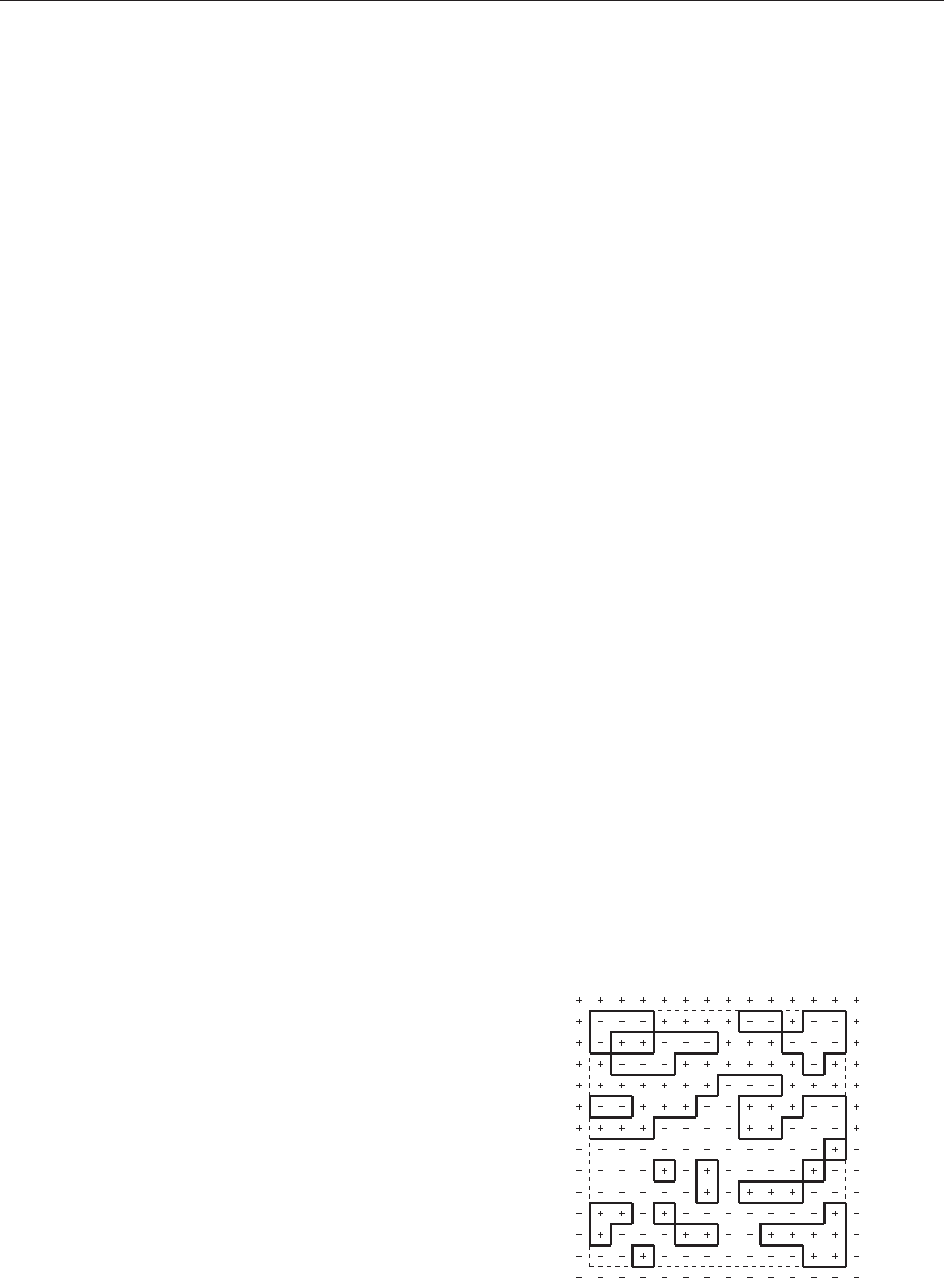
(see Figure 2); or (2) the boundary conditions in
AOB
Figure 2 The dashed line is the boundary of ; the outer spins
correspond to the boundary condition. The points A, B are
points where an open ‘‘line’’ ends.
70 Introductory Article: Equilibrium Statistical Mechanics

which some of the opposite sides of are
identified while þ or conditions are assigned on
the remaining sides: call these ‘‘cylindrical or
semiperiodic boundary conditions.’’
A new description of the spin configurations is
useful: given s, draw a unit segment perpendicular
to the center of each bond b having opposite spins at
its extremes. An example of this construction is
provided by Figure 2 for the boundary condition .
The set of segments can be grouped into lines
separating regions where the spins are positive from
regions where they are negative. If the boundary
condition is þ or , the lines form ‘‘closed polygons’’,
whereas, if the condition is , there is also a single
polygon
1
which is not closed (as in Figure 2). If the
boundary condition is periodic or cylindrical, all
polygons are closed but some may ‘‘go around’’ .
The polygons are also called ‘‘con tours’’ and the length
of a polygon will be denoted jj.
The correspondence (
1
,
2
, ...,
n
,
1
) ! s, for
the boundary condition or, for the boundary
condition þ (or ), s ! (
1
, ...,
n
) is one-to-one
and, if h = 0, the energy H
(s) of a configuration is
higher than J(number of bonds in )byan
amount 2J(j
1
jþ
P
i
j
i
j) or, respectively, 2J
P
i
j
i
j.
The grand canonical probability of each spin
configuration is therefore proportional, if h = 0,
respectively, to
e
2Jðj
1
jþ
P
i
j
i
jÞ
or e
2J
P
i
j
i
j
½45
and the ‘‘up–down’’ symmetry is clearly reflected
by [45].
The average h
x
i
,þ
of
þ
with þ boundary
conditions is given by h
x
i
,þ
= 1 2P
,þ
(), where
P
,þ
() is the probability that the spin
x
is 1. If the
site x is occupied by a negative spin then the point x is
inside some contour associated with the spin
configuration s under consideration. Hence, if ()
is the probability that a given contour belongs to
the set of contours describing a configuration s,it
is P
,þ
()
P
ox
()whereox means that
‘ ‘ surrounds’’ x.
If =(
1
, ...,
n
) is a spin configuration and if
the symbol comp means that the contour is
‘‘disjoint’’ from
1
, ...,
n
(i.e., { [ } is a new spin
configuration), then
ðÞ¼
P
3
e
2J
P
0
2
j
0
j
P
e
2J
P
0
2
j
0
j
e
2Jjj
P
comp
e
2J
P
0
2
j
0
j
P
e
2J
P
0
2
j
0
j
e
2Jjj
½46
because the last ratio in [46] does not exceed 1.
Note that there are >3
p
different shapes of with
perimeter p and at most p
2
congruent ’s containing
x; therefore, the probability that the spin at x is
when the boundary condition is þ satisfies the
inequality
P
;þ
ðÞ
X
1
p¼4
p
2
3
p
e
2Jp
!
!1
0
This probability can be made arbitrarily small so
that h
x
i
,þ
is estimated by a quantity which is as
close to 1 as desired provided is large enough and
the closeness of h
x
i
,þ
to 1 is estimated by a
quantity which is both x and independen t.
A similar argument for the ()-boundary condition,
or the remark that for h = 0itish
x
i
,
= h
x
i
,þ
,
leads to conclude that, at large , h
x
i
,
6¼h
x
i
,þ
and the difference between the two quantities
is positive uniformly in . This is the proof
(Peierls’ theorem)ofthefactthatthereis,if is
large, a strong instability, of the magnetization with
respect to the boundary conditions, i.e., the nearest-
neighbor Ising model in dimension 2 (or greater, by an
identical argument) has a phase transition. If the
dimension is 1, the argument clearly fails and no phase
transition occurs (see the section ‘ ‘Absence of phase
transitions: d = 1’’).
For more details, see Gallavotti (1999).
Finite-Volume Effects
The description in the last section of the phase
transition in the nearest-neighbor Ising model can be
made more precise both from physical and mathe-
matical points of view giving insights into the nature
of the phase transitions. Assume that the boundary
condition is the (þ)-boundary condition and
describe a spin configuration s by means of the
associated closed disjoint polygons (
1
, ...,
n
).
Attribute to s = (
1
, ...,
n
) a probability propor-
tional to [45]. Then the following Minlos–Sinai’s
theorem holds:
Theorem If is large enough there exist C > 0,
() > 0 with () e
2Jjj
and such that a spin
configuration s randomly chosen out of the grand
canonical distribution with þ boundary conditions
and h = 0 will contain, with probability approaching
1 as !1, a number K
()
(s) of contours con-
gruent to such that
jK
ðÞ
ðsÞðÞjjj C
ffiffiffiffiffiffiffi
jj
p
e
Jjj
½47
and this relation holds simultaneously for all ’s.
Introductory Article: Equilibrium Statistical Mechanics 71
Thus, there are very few contours (and the larger
they are the smaller is, in absolute and relative
value, their number): a typical spin configuration in
the grand canonical ensemble with (þ)-boundary
conditions is such that the large majority of the spins
is ‘‘positive’’ and, in the ‘‘sea’’ of positive spins, there
are a few negative spins distributed in small and
rare regions (their number, however, is still of order
of jj).
Another consequence of the analysis in the last
section concerns the the approximate equation of
state near the phase transition region at low
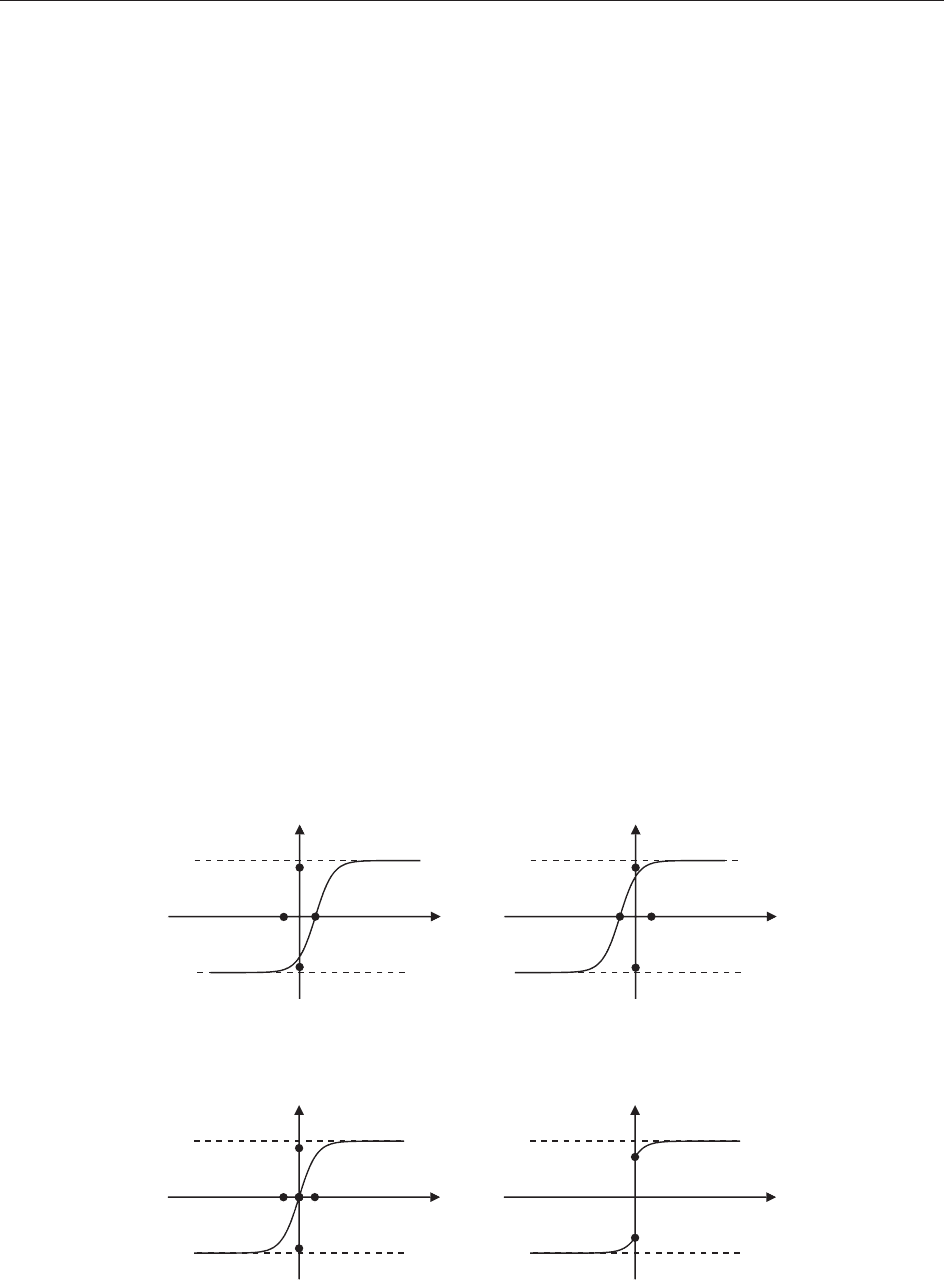
temperatures and finite .If is finite, the graph
of h versus m
(, h) will have a rather different
behavior depending on the possible boundary con-
ditions. For example, if the boundary condition is
(þ)or(), one gets, respectively, the results
depicted in Figure 3a and 3b, where m
() denotes
the spontaneous magnetization (i.e., m
() =
def
lim
h!0
þ
lim
!1
m
(, h)).
With periodic or empty boundary conditions, the
diagram changes as in Figure 4. The thermody-
namic limit m(, h) = lim
!1
m
(, h) exists for all
h 6¼ 0 and the resulting graph is in Figure 4b,
which shows that at h = 0 the limit is discontin-
uous. It can be proved, if is large enough, that
1 > lim
h !0
þ
@
h
m(, h) = () > 0(i.e.,theangle
between the vertical part of the graph and the rest
is sharp).
Furthermore, it can be proved that m(, h)is
analytic in h for h 6¼ 0. If is small enough,
analyticity holds at all h. For large, the function
f (, h) has an essential singularity at h = 0: a result
that can be interpreted as excluding a naive theory
of metastability as a description of states governed
by an equation of state obtained from an analytic
continuation to negative values of h of f (, h).
The above considerations and results further
clarify t he meaning of a phase transition for a
finite system. For more details, we refer the
reader to Gallavotti (1999) and Friedli and Pfister
(2004).
Beyond Low Temperatures
(Ferromagnetic Ising Model)
A limitation of the results discussed above is the
condition of low temperature (‘‘ large enough’’).
A natural problem is to go beyond the low-
temperature region and to describe fully the phe-
nomena in the region where boundary condition
instability takes place and first develops. A number
of interesting partial results are known, which
considerably improve the picture emerging from
the previous analysis. A striking list, but far from
exhaustive, of such results follows and focuses on
the properties of ferromagnetic Ising spin systems.
The reason for restricting to such cases is that they
are simple enough to allow a rather fine analysis,
which sheds consi derable light on the structure of
statistical mechanics suggesting precise formulation
h
m
Ω
(β, h)
m*(β)
–m*(β)
–O(|Ω|
–1/2
)
O(|Ω|
–1/2
)
h
1
m*(β)
–m*(β)
O
(|Λ|
–1/2
)
–O
(|Λ|
–1/2
)
m
Ω
(β, h)
1
(a)
(b)
Figure 3 The h vs m
(, h) graphs for finite and (a) þ and (b) conditions.
m
Ω
(β, h)
m*(β)
–m*(β)
–O(|Ω|
–1/2
)
O(|Ω|
–1/2
)
h
1
m*(β)
–m*(β)
m(β, h)
h
1
(a)
(b)
Figure 4 (a) The h vs m
(, h) graph for periodic or empty boundary conditions. (b) The discontinuity (at h = 0) of the thermodynamic limit.
72 Introductory Article: Equilibrium Statistical Mechanics

of the problems that it would be desirable to
understand in more general syst ems.
1. Let z =
def
e
h
and consid er that the product of z
V
(V is the number of sites jj of ) times the
partition function with periodic or perfect-wall
boundary condit ions and with finite-range
ferromagnetic interaction, not necessarily nearest-
neighbor; a polynomial in z (of degree 2V)
is thus obtained. Its zeros lie on the unit
circle jzj= 1: this is Lee–Yang’s theorem.It
implies that the only singularities of f (, h)in
the region 0 <<1, 1 < h < þ1 can be
found at h = 0.
A singularity can appear only if the point z = 1
is an accumulation point of the limiting distribu-
tion (as !1) of the zeros on the unit circle: if
the zeros are z
1
, ..., z
2V
then
1
V
log z
V
Zð; h; ; periodicÞ
¼ 2J þ h þ
1
V
X
2V
i¼1
logðz z
i
Þ
and if
V
1
ðnumber of zeros of the form
z
j
¼ e
i
j
;
j
þ dÞ!
!1
d
ðÞ
2
it is
f ð; hÞ¼2J þ
1
2
Z
logðz e
i
Þd
ðÞ½48
The existence of the measure d
() follows from
the existence of the thermodynamic limit: but
d
() is not necessarily d-continuous, i.e., not
necessarily proportional to d.
2. It can be shown that, with not necessarily a
nearest-neighbor interaction, the zeros of the
partition function do not move too much under
small perturbations of the potential even if one
perturbs the energy (at perfect-wall or periodic
boundary conditions) into
H
0
ðsÞ¼H
ðsÞþðH
ÞðsÞ
ðH
ÞðsÞ¼
X
X
J
0
ðXÞ
X
½49
where J
0
(X) is very general and defined on
subsets X = (x
1
, ..., x
k
) such that the quan-
tity jjJ
0
jj= sup
y2Z
d
P
y2X
jJ
0
(X)j is small enough.
More precisely, with a ferromagnetic pair
potential J fixed, suppose that one knows that,
when J
0
= 0, the partition function zeros in the
variable z = e
h
lieinacertainclosedsetN (of
the unit circle) in the z-plane. Then, if J
0
6¼ 0,
they lie in a closed set N
1
, -independent and
contained in a neighborhood of N of width
shrinking to 0 when jjJ
0
jj ! 0. This allows to
establish various relations between analyticity
properties and boundary condition instability
as described in (3) below.
3. In the ferromagnetic Ising model, with not necessa-
rily a nearest-neighbor interaction, one says that
thereisagaparound0ifd
() = 0near = 0. It
can be shown that if is small enough there is a gap
for all h of width uniform in h.
4. Another question is whether the boundary
condition instability is always revealed by the
one-spin correlation function (i.e., by the magne-
tization) or whether it might be shown only
by some correlation functions of higher order. It
can be proved that no boundary condition
instability occurs for h 6¼ 0; at h = 0 it is possible
only if
lim
h!0
mð; hÞ 6¼ lim
h!0
þ
mð; hÞ½50
5. A consequence of the Griffiths’ inequalities
(cf. the section ‘‘Thermodynamic limits and
inequalities’’) is that if [50] is true for a given
0
then it is true for all >
0
. Therefore, item
(4) leads to a natural definition of the critical
temperature T
c
as the least upper bound of the
T ’s such that [50] holds (k
B
T =
1
).
6. If d = 2 the free energy of the nearest-neighbor
ferromagnetic Ising model has a singularity
at
c
and the value of
c
is known exactly
from the exact solutions of the model:
m(,0
þ
) =
def
m
() (1 sinh
4
2J)
1=8
. The loca-
tion and nature of the singularities of f (,0) as a
function of remains an open question for d = 3.
In particular, the question whether there is a
singularity of f (,0) at =
c
is open.
7. For <
c
there is instability with respect to
boundary conditions (see (6) above) and a
natural question is: how many ‘‘pure’’ phases
can exist in the ferromagnetic Ising model?
(cf. the section ‘‘Phase trans itions and boundary
conditions,’’ eqn [22]). Intuitio n suggests
that there should be only two phases: the
positively magnetized and the negatively
magnetized ones.
One has to distinguish between translation-
invariant pure phases and non-translation-invariant
ones. It can be proved that, in the case of the
two-dimensional nearest-neighbor ferromagnetic
Ising models, all infinite-volume states (cf. the
section ‘‘Lattice models’’) are translationally invar-
iant. Furthermore, they can be obtained by
Introductory Article: Equilibrium Statistical Mechanics 73

considering just the two boundary conditions þ
and : the latter states are also pure states for
models with non-nearest-neighbor ferromagnetic
interaction. The solution of this problem has led to
the introduction of many new ideas and techniques
in statistical mechanics and probability theory.
8. In any dimension d 2, for large enough, it can
be proved that the nearest-neighbor Ising model
has only two translation-invariant phases. If the
dimension is 3 and is large, the þ and
phases exhaust the set of translation-invariant
pure phases but there exist non-translation-
invariant phases. For close to
c
, however, the
question is much more difficult.
For more details, see Onsager (1944), Lee and
Yang (1952), Ruelle (1971), Sinai (1991), Gallavotti
(1999), Aizenman (1980), Higuchi (1981), and
Friedli and Pfister (2004).
Geometry of Phase Coexistence
Intuition about the phenomena connect ed with the
classical phase transitions is usually based on the
properties of the liquid–gas phase transition; this
transition is usually experimentally investigated in
situations in which the total number of particles is
fixed (canonical ensemble) and in presence of an
external field (gravity).
The importanc e of such experimental conditions
is obvious; the external field produces a nontransla-
tionally invariant situation and the corresponding
separation of the two phases. The fact that the
number of particles is fixed determines, on the other
hand, the fraction of volume occupied by each of the
two phases.
Once more, consider the nearest-neighbor ferro-
magnetic Ising model: the results available for it can
be used to obtain a clear picture of the solution to
problems that one would like to solve but which in
most other models are intractable with present-day
techniques.
It will be convenient to discuss phase coexistence in
the canonical ensemble distributions on configurations
of fixed total magnetization M = mV (see the section
‘ ‘Lattice models’ ’; [40]). Let be large enough to be in
the two-phase region and, for a fixed 2 (0, 1), let
m ¼ m
ðÞþð1 Þðm
ðÞÞ
¼ð1 2Þm
ðÞ½51
that is, m is in the vertical part of the diagram
m = m(, h)at fixed (see Figure 4).
Fixing m as in [51] does not yet determin e the
separation of the phases in two different regions; for
this effect, it will be necessary to introduce some
external cause favoring the occupation of a part of
the vo lume by a single phase. Such an asymmetry
can be obtained in at least two ways: through a
weak uniform external field (in complete analogy with
the gravitational field in the liquid–vapor transition) or
through an asymmetric field acting only on boundary
spins. The latter should have the same qualitative
effect as the former, because in a phase transition
region a boundary perturbation produces volume
effects (see sections ‘ ‘Phase transitions and inequal-
ities’ ’ and ‘ ‘Symmetry-breaking phase transitions’ ’).
From a mathematical point of view, it is simpler to
use a boundary asymmetry to produce phase separa-
tions and the simplest geometry is obtained by
considering -cylindrical or þþ-cylindrical boundary
conditions: this means þþ or boundary conditions
periodic in one direction (e.g., in Figure 2 imagine the
right and left boundary identified after removing the
boundary spins on them).
Spins adjacent to the bases of act as symmetry-
breaking external fields. The þþ-cylindrical bound-
ary con dition should favor the formation inside
of the positively magnetized phase; therefore, it
will be natural to consider, in the canonical
distribution, this boundary condition only when
the total magnetization is fixed to be the sponta-
neous magnetization m
().
On the other hand, the -boundary condition
favors the separation of phases (positively magnetized
phase near the top of and negatively magnetized
phase near the bottom). Therefore, it will be natural
to consider the latter boundary condition in the
case of a canonical distribution with magnetization
m = (1 2)m
()with0<<1([51]). In the latter
case, the positive phase can be expected to adhere to
the top of and to extend, in some sense to be
discussed, up to a distance O(L) from it; and then to
change into the negatively magnetized pure phase.
To make the phenomenological description
precise, consider the spin configurations s through
the associated sets of disjoint polygons (cf. the
section ‘‘Symmetry-breaking phase transitions’’). Fix
the boundary conditions to be þþ or -cylindrical
boundary conditions and note that polygons asso-
ciated with a spin configuration s are all closed and
of two types: the ones of the first type, denoted
1
, ...,
n
, are polygons which do not encircle ; the
second type of polygons, denoted by the symbols
,
are the ones which wind up, at least once, around .
So, a spin configuration s will be described by a set
of polygons; the statistical weight of a configuration
s = (
1
, ...,
n
,
1
, ...,
h
)is(cf.[45]):
e
2J
P
i
j
i
jþ
P
j
j
j
j
½52
74 Introductory Article: Equilibrium Statistical Mechanics