Francoise J.-P., Naber G.L., Tsun T.S. (editors) Encyclopedia of Mathematical Physics
Подождите немного. Документ загружается.

triplet can hop from link to link, creating a gapped
‘‘triplon’’ quasiparticle excitation. This is similar to
the large g paramagnet for H
I
, with the important
difference that each quasiparticle is now 3-fold
degenerate.
At g = 1, the ground state of H
d
is not known
exactly. However, at this point H
d
becomes equiva-
lent to the nearest-neighbor square lattice antiferro-
magnet, and this is known to have antiferromagnetic
order in the ground state, as illustrated in Figure 4.
This state is similar to the ferromagnetic ground
state of H
I
, with the difference that the magnetic
moment now acquires a staggered pattern on the
two sublattices, rather than the uniform moment of
the ferromagnet. Thus, in this ground state
hAFj^
j
jAFi¼N
0
j
n
½10
where 0 < N
0
< 1 is the antiferromagnetic moment,
j
= 1 identifies the two sublattices in Figure 4, and
n
is an arbitrary unit vector speci fying the
orientation of the spontaneous magnetic moment
which breaks the O(3) spin rotation invariance of
H
d
. The excitations above this antiferromagnet are
also distinct from those of the paramagnet: they are
a doublet of spin waves consisting of a spatial
variation in the local orientation, n
, of the
antiferromagnetic order: the energy of this excita-
tion vanishes in the limit of long wavelengths, in
contrast to the finite energy gap of the triplon
excitation of the paramagnet.
As with H
I
, we can conclude from the distinct
characters of the ground states and excitations for
g 1andg 1 that there must be a quantum
critical point at some intermediate g = g
c
.
Quantum Criticality
The simple considerations of the previous section
have given a rather complete descr iption (based on
the quasiparticle picture) of the physics for g g
c
and g g
c
. We turn, finally, to the region g g
c
.
For the specific models discussed in the previous
section, a useful description is obtained by a method
that is a generalization of the LGW method
developed earlier for thermal phase transitions.
However, some aspects of the critical behavior
(e.g., the general forms of eqns [13]–[15]) will
apply also to the quantum critical point of the
section ‘‘Beyond LGW theory.’’
Following the canonical LGW strategy, we need
to identify a collectiv e order parameter which
distinguishes the two phases. This is clearly given
by the ferromagnetic moment in eqn [4] for the
quantum Ising chain, and the antiferromagnetic
moment in eqn [10] for the coupled dimer antiferro-
magnet. We coarse-grain these moments over some
finite averaging region, and at long wavelengths this
yields a real order parameter field
a
, with the index
a = 1, ..., n. For the Ising case we have n = 1 and
a
is a measure of the local average of N
0
as defined in
eqn [4]. For the antiferromagnet, a extends over the
three values x, y, z (so n = 3), and three components
of
a
specify the magnitude and orientation of the
local antiferromagnetic order in eqn [10]; note the
average orientation of a specific spin at site j is
j
times the local value of
a
.
The second step in the LGW approach is to write
down a general field theory for the order parameter,
consistent with all symmetries of the underlying
model. As we are dealing with a quantum transition,
the field theory has to extend over spacetime, with
the temporal fluctuations representing the sum over
histories in the Feynman path-integral approach.
With this reasoni ng, the proposed partition function
(
=
–
)/
√2
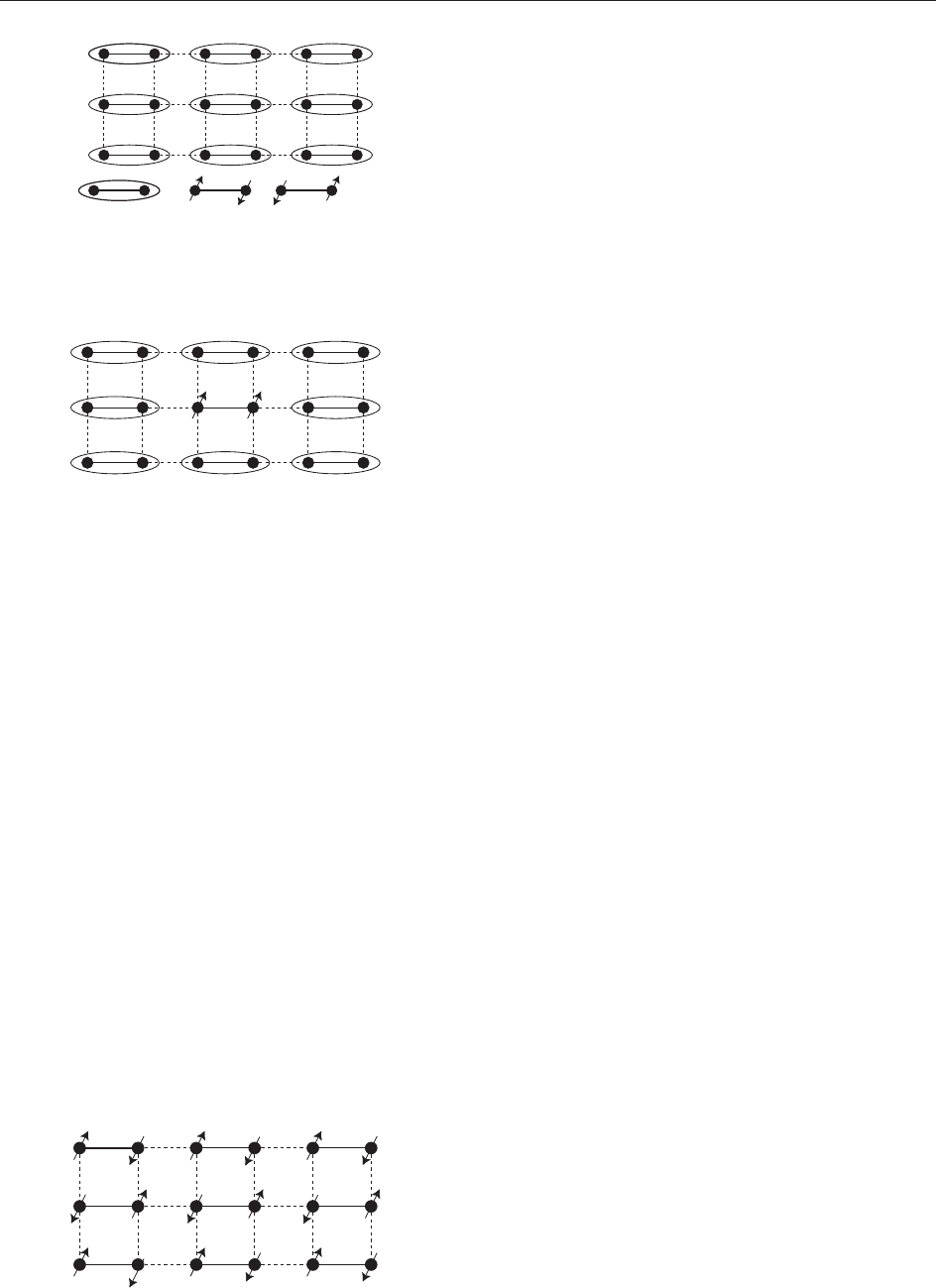
Figure 2 The paramagnetic state of H
d
for g > g
c
. The state
illustrated is the exact ground state for g = 1, and it is
adiabatically connected to the ground state for all g > g
c
.
Figure 3 The triplon excitation of the g > g
c
paramagnet. The
stationary triplon is an eigenstate only for g = 1 but it becomes
mobile for finite g.
Figure 4 Schematic of the ground state with antiferromagnetic
order with g < g
c
.
292 Quantum Phase Transitions
for the vicinity of the critical point takes the
following form:
Z
¼
Z
D
a
ðx;Þ
exp
Z
d
d
x d
1
2
ð@
a
Þ
2
þc
2
ðr
x
a
Þ
2
þ s
2
a
þ
u
4!
2
a
2
½11
Here is imaginary time; there is an implied
summation over the n values of the index a, c is a
velocity, and s and u > 0 are coupling constants.
This is a field theory in d þ 1 spacetime dimensions,
in which the Ising chain corresponds to d = 1 and
the dimer antiferromagnet to d = 2. The quantum
phase transition is accessed by tuning the ‘‘mass’’ s:
there is a quantum critical point at s = s
c
and the
s < s
c
(s > s
c
) regions correspond to the g < g
c
(g > g
c
)
regions of the lattice models. The s < s
c
phase has
h
a
i6¼0 and this corresponds to the spontaneous
breaking of spin rotation symmetry noted in eqns [4]
and [10] for the lattice models. The s > s
c
phase is
the paramagnet with h
a
i=0. The excitat ions in this
phase can be unde rstood as small harmonic oscilla-
tions of
a
about the point (in field space)
a
=0. A
glance at eqn [11] shows that there are n such
oscillators for each wave vector. These oscillators
clearly constitute the g > g
c
quasiparticles found
earlier in eqn [7] for the Ising chain (with n= 1)
and the triplon quasiparticle (with n =3) illustrated
in Figure 3 for the dimer antiferromagnet.
We have now seen that there is a perfect
correspondence between the phases of the quantum
field theory Z
and those of the lattice models H
I
and H
d
. The power of the representation in eqn [11]
is that it also allows us to get a simple description of
the quantum critical point. In particular, readers
may already have noticed that if we interpret the
temporal direction in eqn [11] as another spatial
direction, then Z
is simply the classical partition
function for a thermal phase transition in a ferro-
magnet in d þ 1 dimensions: this is the canonical
model for which the LGW theory was originally
developed. We can now take over standard results
for this classical critical point, and obtain some
useful predictions for the quantum critical point of
Z
. It is useful to express these in terms of the
dynamic susceptibility defined by
ðk;!Þ¼
i
h
Z
d
d
x
Z
1
0
dt
^
ðx; tÞ;
^
ð0; 0Þ
hiDE
T
e
ikxþi!t
½12
Here
^
is the Heisenberg field operator correspond-
ing to the path integral in eqn [11], the square
brackets represent a commutator, and the angular
brackets an average over the partition function at a
temperature T. The structure of can be deduced
from the knowledge that the quantum correlators of
Z
are related by analytic continuation in time to
the corresponding correlators of the classical statis-
tical mech anics problem in d þ 1 dimensio ns. The
latter are known to diverge at the critical point as
1=p
2
where p is the (d þ 1)-dimensional momen-
tum, is defined to be the anomalous dimension of
the order parameter ( = 1=4 for the quantum Ising
chain). Knowing this, we can deduce the form of the
quantum correlator in eqn [12] at the zero-tempera-
ture quantum critical point
ðk;!Þ
1
ðc
2
k
2
!
2
Þ
1=2
; T ¼ 0; g ¼ g
c
½13
The most important property of eqn [13] is the
absence of a quasiparticle pole in the spectral
density. Instead, Im((k, !)) is nonzero for all !>ck,
reflecting the presence of a continuum of critical
excitations. Thus the stable quasiparticles found at
low enough energies for all g 6¼ g
c
are absent at the
quantum critical point.
We now briefly discuss the nature of the phase
diagram for T > 0 with g near g
c
. In general, the
interplay between quantum and thermal fluctuations
near a quantum critical point can be quite compli-
cated, and we cannot discuss it in any detail here.
However, the physics of the quantum Ising chain is
relatively simple, and also captures many key
features found in more complex situations, and is
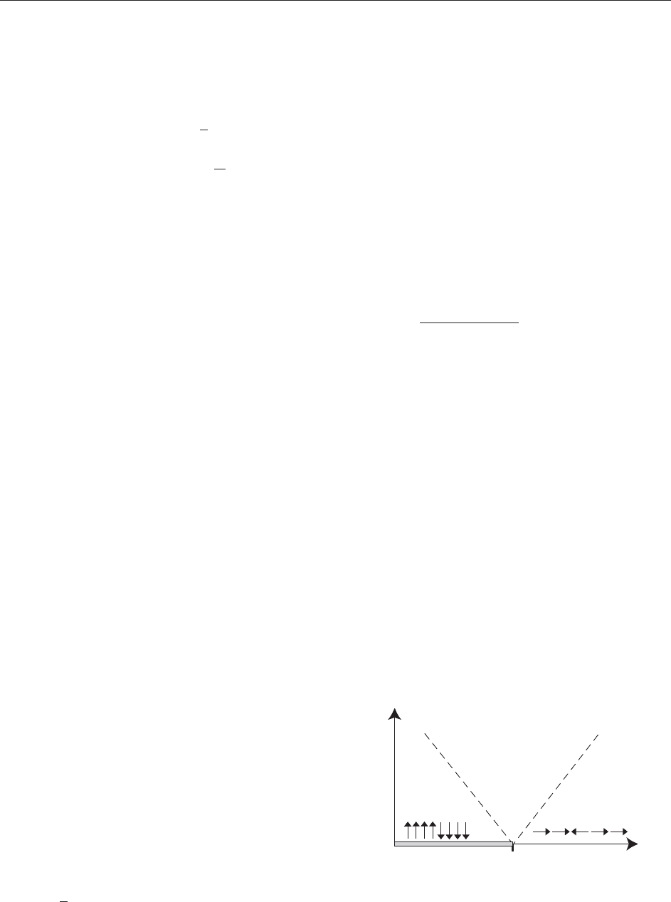
summarized in Figure 5. For all g 6¼ g
c
there is a
range of low temperatures (T
<
jg g
c
j) where the
long time dynamics can be described using a dilute
gas of thermally excited quasiparticles. Further, the
g
T
g
c
0
Domain wall
quasiparticles
Quantum
critical
Flipped-spin
quasiparticles
Figure 5 Nonzero temperature phase diagram of H
I
: The
ferromagnetic order is present only at T = 0 on the shaded line
with g < g
c
: The dashed lines at finite T are crossovers out of
the low-T quasiparticle regimes where a quasiclassical descrip-
tion applies. The state sketched on the paramagnetic side used
the notation !ji
j
= 2
1=2
( "ji
j
þ#ji
j
) and ji
j
= 2
1=2
( "ji
j
#ji
j
):
Quantum Phase Transitions 293
dynamics of these quasiparticles is quasiclassical,
although we reiterate that the nature of the
quasiparticles is entirely distinct on opposite sides
of the quantum critical point. Most interesting,
however, is the novel quantum critical region,
T
>
jg g
c
j, where neither quasiparticle picture nor
a quasiclassical descr iption are appropriate. Instead,
we have to understand the influence of temperature
on the critical continuum associated with eqn [13].
This is aided by scaling arguments which show that
the only important frequency scale which charac-
terizes the spectrum is k
B
T=h, and the crossovers
near this scale are universal, that is, independent of
specific microscopic details of the lattice Hamilto-
nian. Consequently, the zero-momentum dynamic
susceptibility in the quantum critical region takes
the following form at small frequen cies:
ðk ¼ 0;!Þ
1
T
2
1
ð1 i!=
R
Þ
½14
This has the structure of the respons e of an
overdamped osci llator, and the damping frequency,
R
, is given by the universal expression
R
¼ 2 tan
16
k
B
T
h
½15
The numerical proportionality constant in eqn. [15]
is specific to the quantum Ising chain; other models
also obey eqn [15] but with a different numerical
value for this constant.
Beyond LGW Theory
The quantum transitions discussed so far have
turned to have a critical theory identical to that
found for classical thermal transitions in d þ 1
dimensions. Over the last decade it ha s become
clear that there are numerous models, of key
physical importance, for which such a simple
classical correspondence does not exist. In these
models, quantum Berry phases are crucial in estab-
lishing the nature of the phases, and of the critical
boundaries between them. In less technical terms, a
signature of this subtlety is an important simplifying
feature which was crucial in the analyses of the
section ‘‘Simple models’’: both models had a
straightforward g !1limit in which we were able
to write down a simple, nondegenerate, gro und-state
wave function of the ‘‘disordered’’ paramagnet. In
many other models, identification of the disordered
phase is not as straightforward: specifying absence
of a particular magnetic order is not enough to
identify a quantum state, as we still need to write
down a suitable wave function. Often, subtle
quantum interference effects induce new types of
order in the disordered state, and such effects are
entirely absent in the LGW theory.
An important example of a system displaying such
phenomena is the S = 1=2 square lattice antiferro-
magnet with additional frustrating interactions. The
quantum degrees of freedom are identical to those of
the coupled dimer antiferromagnet, but the Hamil-
tonian preserves the full point-group symmetry of
the square lattice:
H
s
¼
X
j<k
J
jk
^
x
j
^
x
k
þ ^
y
j
^
y
k
þ ^
z
j
^
z
k
þ ½16
Here the J
jk
> 0 are short-range exchange interac-
tions which preserve the square lattice symmetry,
and the ellipses represent possible further multiple
spin terms. Now imagine tuning all the non-nearest-
neighbor terms as a function of some generic
coupling constant g. For small g, when H
s
is nearly
the square lattice antiferromagnet, the ground state
has antiferromagnetic order as in Figure 4 and
eqn [10]. What is now the disordered ground state
for large g? One natural candidate is the spin-singlet
paramagnet in Figure 2. However, because all
nearest neighbor bonds of the square lattice are
now equiva lent, the state in Figure 2 is degenerate
with three other states obtained by successive 90
rotations about a lattice site. In other words, the
state in Figure 2, when transferred to the square
lattice, breaks the symmetry of lattice rotations by
90
. Consequently it has a new type of order, often
called valence-bond-solid (VBS) order. It is now
believed that a large class of model s like H
s
do
indeed exhibit a second-order quantum phase
transition between the antiferromagnetic state and
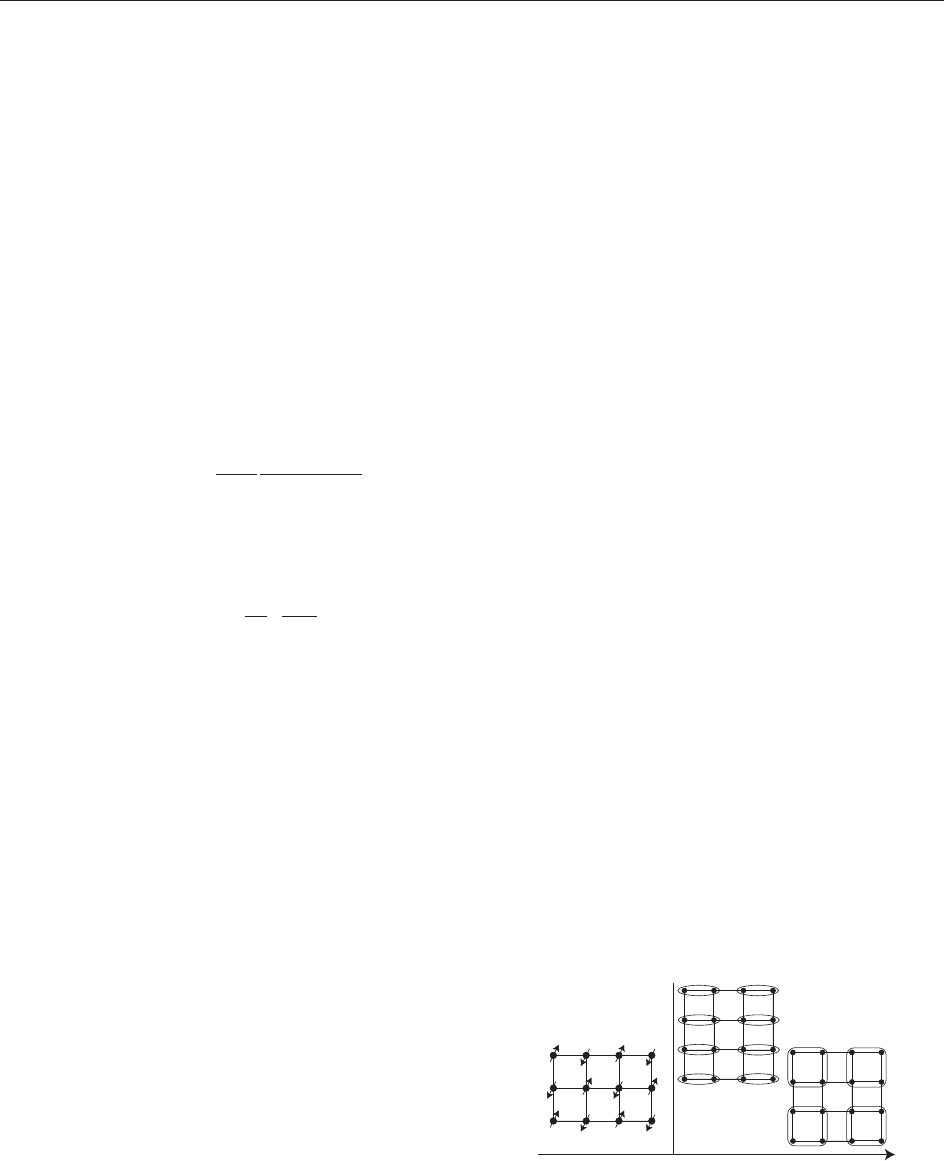
a VBS state – see Figure 6. Both the existence of VBS
order in the paramagnet, and of a second-order
quantum transition, are features that are not
predicted by LGW theory: these can only be
g
g
c
or
Antiferromagnetic
order
VBS order
Figure 6 Phase diagram of H
s
. Two possible VBS states are
shown: one which is the analog of Figure 2, and the other in
which spins form singlets in a plaquette pattern. Both VBS states
have a 4-fold degeneracy due to breaking of square lattice
symmetry. So the novel critical point at g = g
c
(described by Z
z
)
has the antiferromagnetic and VBS orders vanishing as it is
approached from either side: this coincident vanishing of orders
is generically forbidden in LGW theories.
294 Quantum Phase Transitions

understood by a careful study of quantum inter-
ference effects associated with Berry phases of spin
fluctuations about the antiferromagnetic state. We
will not enter into details of this analysis here, but will
conclude our discussion by writing down the theory so
obtained for the quantum critical point in Figure 6:
Z
z
¼
Z
Dz
ðx;ÞDA
ðx;Þ
exp
Z
d
2
x d
jð@
iA
Þ
z
j
2
þ sjz
j
2
þ
u
2
ðjz
j
2
Þ
2
þ
1
2e
2
ð
@
A
Þ
2
½17
Here , , are spacetime indices which extend over
the two spatial directions and , is a spinor index
which extends over ", #, and z
is complex spinor
field. In comparing Z
z
to Z
, note that the vector
order parameter
a
has been replaced by a spinor z
,
and these are related by
a
= z
a
z
, where
a
are
the Pauli matrices. So the order parameter has
fractionalized into the z
. A second novel property
of Z
z
is the presence of a U(1) gauge field A
: this
gauge force emerges near the critical point, even
though the underlying model in eqn [16] only has
simple two spin interactions. Studies of fractiona-
lized critical theories like Z
c
in other models with
spin and/or charge excitations is an exciting avenue
for further theoretical research.
See also: Bose–Einstein Condensates; Boundary
Conformal Field Theory; Fractional Quantum Hall Effect;
Ginzburg–Landau Equation; High Tc Superconductor
Theory; Quantum Central-Limit Theorems; Quantum
Spin Systems; Quantum Statistical Mechanics: Overview.
Further Reading
Matsumoto M, Yasuda C, Todo S, and Takayama H (2002)
Physical Review B 65: 014407.
Sachdev S (1999) Quantum Phase Transitions. Cambridge:
Cambridge University Press.
Senthil T, Balents L, Sachdev S, Vishwanath A, and Fisher MPA,
http://arxiv.org/abs/cond-mat/0312617.
Quantum Spin Systems
B Nachtergaele, University of California at Davis,
Davis, CA, USA
ª 2006 B Nachtergaele. Published by Elsevier Ltd.
All rights reserved.
Introduction
The theory of quantum spin systems is concerned with
the properties of quantum systems with an infinite
number of degrees of freedom that each have a finite-
dimensional state space. Occasionally, one is specifically
interested in finite systems. Among the most common
examples, one has an n-dimensional Hilbert space
associated with each site of a d-dimensional lattice.
A model is normally defined by describing
a Hamiltonian or a family of Hamiltonians, which
are self-adjoint operators on the Hilbert space, and
one studies their spectrum, the eigenstates, the
equilibrium states, the system dynamics, and non-
equilibrium stationary states, etc.
More particularly, the term ‘‘quantum spin sys-
tem’’ often refers to such models where each degree
of freedom is thought of as a spin variab le, that is,
there are three basic observables representing the
components of the spin, S
1
, S
2
,andS
3
, and these
components transform according to a unitary repre-
sentation of SU(2). The most comm only encountered
situation is where the system consi sts of N spins, each
associated with a fixed irreducible representation of
SU(2). One speaks of a spin-J model if this represen-
tation is the (2J þ 1)-dimensional one. The possible
values of J are 1/2, 1, 3/2, ...
The spins are usually thought of as each being
associated with a site in a lattice, or more generally, a
vertex in a graph. In a condensed-matter-physics
model, each spin may be associated with an ion in a
crystalline lattice. Quantum spin systems are also used
in quantum information theory and quantum compu-
tation, and show up as abstract mathematical objects
in representation theory and quantum probability.
In this article we give a brief introduction to the
subject, starting with a very short review of its history.
The mathematical framework is sketched and the most
important definitions are given. Three sections, ‘‘Sym-
metries and symmetry breaking,’ ’ ‘ ‘Phase transitions,’’
and ‘ ‘Dynamics,’’ together cover the most important
aspects of quantum spin systems actively pursued today.
A Very Brief History
The introduction of quantum spin systems was the
result of the marriage of two developments during
the 1920s. The first was the realization that angular
momentum (hence, also the magnetic moment) is
quantized (Pauli 1920, Stern and Gerlach 1922) and
that particles such as the electron have an intrinsic
Quantum Spin Systems 295

angular momentum called spin (Compton 1921,
Goudsmit and Uhlenbeck 1925).
The second development was the attempt in
statistical mechanics to explain ferromagnetism and
the phase transition associated with it on the basis of a
microscopic theory (Lenz and Ising 1925). The
fundamental interaction between spins, the so-called
exchange operator which is a subtle consequence
of the Pauli exclusion principle, was introduced
independently by Dirac and Heisenberg in 1926.
With this discovery, it was realized that magnetism is
a quantum effect and that a fundamental theory
of magnetism requires the study of quantum-mechan-
ical models. This realization and a large amount of
subsequent work notwithstanding, some of the most
fundamental questions, such as a derivation of
ferromagnetism from first principles, remain open.
The first and most important quantum spin model
is the Heisenberg model, so named after Heisenberg.
It has been studied intensely ever since the early
1930s and its study has led to an impressive variety
of new ideas in both mathematics and physics. Here,
we limit ourselves to listing only some landmark
developments.
Spin waves were discovered independently by
Bloch and Slater in 1930 and they continue to play
an essential role in our understanding of the
excitation spectrum of quantum spin Hamiltonians.
In two papers published in 1956, Dyson advanced
the theory of spin waves by showing how interac-
tions between spin waves can be taken into account.
In 1931, Bethe introduced the famous Bethe
ansatz to show how the exact eigenvectors of the
spin-1/2 Heisenberg model on the one-di mensional
lattice can be found. This exact solution, directly
and indirectly, led to many important developments
in statistical mechanics, combinatorics, representa-
tion theory, quantum field theory and more.
Hulthe´n used the Bethe ansatz to compute the
ground-state energy of the antiferromagnetic spin-
1/2 Heisenberg chain in 1938.
In their famous 1961 paper, Lieb, Schultz, and
Mattis showed that some quantum spin models in
one dimension can be solved exactly by mapping
them into a problem of free fermions. This paper is
still one of the most cited in the field.
Robinson, in 1967, laid the foundation for the
mathematical framework, which we describe in the
next section. Using this framework, Araki estab-
lished the absence of phase transitions at positive
temperatures in a large class of one-dimens ional
quantum spin models in 1969.
During the more recent decades, the mathematical
and computational techniques used to study quantum
spin models have fanned out in many directions.
When it was realized in the 1980s that the magnetic
properties of complex materials play an important role
in high-T
c
superductivity, a variety of quantum spin
models studied in the literature proliferated. This
motivated a large number of theoretical and experi-
mental studies of materials with exotic properties that
are often based on quantum effects that do not have a
classical analog. An example of unexpected behavior is
the prediction by Haldane of the spin liquid ground
state of the spin-1 Heisenberg antiferromagnetic chain
in 1983. In the quest for a mathematical proof of this
prediction (a quest still ongoing today), Affleck,
Kennedy, Lieb, and Tasaki introduced the AKLT
model in 1987. They were able to prove that the
ground state of this model has all the characteristic
properties predicted by Haldane for the Heisenberg
chain: a unique ground state with exponential decay of
correlations and a spectral gap above the ground state.
There are also particle models that are defined on
a lattice, or more generally, a graph. Unlike spins,
particles can hop from one site to another. These
models are closely related to quantum spin systems
and, in some cases, are mathematically equivalent.
The best-known example of a model of lattice
fermions is the Hubbard model. Such systems are
not discussed further in this article.
Mathematical Framework
Quantum spin systems present an area of mathema-
tical physics where the demands of mathematical
rigor can be fully met and, in many cases, this can be
done without sacrificing the ability to include all
physically relevant models and phenomena. This
does not mean, however, that there are few open
problems remaining. But it does mean that, in
general, these open problems are precisely formu-
lated mathematical questions.
In this section we review the standard mathema-
tical framework for quantum spin systems, in which
the topics discussed in the subsequent section can be
given a precise mathematical formulation. It is
possible, however, to skip this section and read the
rest with only a physical or intuitive understanding
of the notions of observable, Hamiltonian,
dynamics, symmetry, ground state, etc.
The most common mathemati cal setup is as follows.
Let d 1, and let L denote the family of finite subsets
of the d-dimensional integer lattice Z
d
.Forsimplicity
we will assume that the Hilbert space of the ‘ ‘spin’’
associated with each x 2 Z
d
has the same dimension
n 2: H
{x}
ffi C
n
. The Hilbert space associated with
the finite volume 2Lis then H
=
N
x2
H
x
.The
algebra of observables for the spin of site x consists of
the n n complex matrices: A
{x}
ffi M
n
(C). For any
296 Quantum Spin Systems

2L, the algebra of observables for the system in is
given by A
=
N
x2
A
{x}
. The primary observables for
a quantum spin model are the spin-S matrices
S
1
, S
2
,and S
3
,whereS is the half-integer such that
n = 2S þ 1. They are defined as Hermitian matrices
satisfying the SU(2) commutation relations. Instead
of S
1
and S
2
, one often works with the spin-raising
and -lowering operators, S
þ
and S
, defined by the
relations S
1
= (S
þ
þ S
)=2, and S
2
= (S
þ
S
)=(2i). In
terms of these, the SU(2) commutation relations are
½S
þ
; S
¼2S
3
; ½S
3
; S
¼S
½1
where we have used the standard notation for the
commutator for two elements A and B in an algebra:
[A, B] = AB BA. In the standard basis S
3
, S
þ
, and
S
are given by the following matrices:
S
3
¼
S
S 1
.
.
.
S
0
B
B
@
1
C
C
A
S
= (S
þ
)
, and
S
þ
¼
0 c
S
0 c
S1
.
.
.
.
.
.
0 c
Sþ1
0
0
B
B
B
B
B
@
1
C
C
C
C
C
A
where, for m = S, S þ 1, ..., S,
c
m
¼
ffiffiffiffiffiffiffiffiffiffiffiffiffiffiffiffiffiffiffiffiffiffiffiffiffiffiffiffiffiffiffiffiffiffiffiffiffiffiffiffiffiffiffi
SðS þ 1Þmðm 1Þ
p
In the case n = 2, one often works with the Pauli
matrices,
1
,
2
,
3
, simply related to the spin
matrices by
j
= 2S
j
, j = 1, 2, 3.
Most physical observables are expressed as finite
sums and products of the spin matrices
S
j
x
, j = 1, 2, 3, associated with the site x 2 :
S
j
x
¼
O
y2
A
y
with A
x
= S
j
, and A
y
= 1 if y 6¼ x.
The A
are finite-dimensional C
-algebras for the
usual operations of sum, product, and Hermitian
conjugation of matrices and with identity 1
.
If
0
1
, there is a natural embedding of A
0
into A
1
, given by
A
0
ffiA
0
1
1
n
0
A
1
The algebra of local observables is then defined by
A
loc
¼
[
2L
A
Its completion is the C
-algebra of quasilocal
observables, which we will simply denote by A.
The dynamics and symmetries of a quantum spin
model are described by (groups of) automorphisms
of the C
-algebra A, that is, bijective linear trans-
formations on A that preserve the product and
operations. Translation invariance, for example, is
expressed by the translation automorphisms
x
, x 2
Z
d
, which map any subalgebra A
to A
þx
, in the
natural way. They form a repre sentation of the
additive group Z
d
on A.
A translation-invariant interaction, or potential,
defining a quantum spin model, is a map : L!A
with the following properties: for all X 2L,
we have (X) 2A
X
, (X ) = (X)
, and for x 2 Z
d
,
(X þ x) =
x
((X)). An interaction is called finite
range if there exists R > 0 such that (X) = 0
whenever diam(X) > R. The Hamiltonian in is
the self-adjoint element of A
defined by
H
¼
X
X
ðXÞ
For the standard Heisenberg model the interaction is
given by
ðfx; ygÞ ¼ JS
x
S
y
; if jx yj¼1 ½2
and (X) = 0 in all other cases. Here, S
x
S
y
is the
conventional notation for S
1
x
S
1
y
þ S
2
x
S
2
y
þ S
3
x
S
3
y
. The
magnitude of the coupling constant J sets a natural
unit of energy and is irrelevant from the mathema-
tical point of view. Its sign, however, determines
whether the model is ferromagnetic ( J > 0), or
antiferromagnetic (J < 0). For the classical Heisen-
berg model, where the role of S
x
is played by a unit
vector in R
3
, and which can be regarded, after
rescaling by a factor S
2
, as the limit S !1of the
quantum Heisenberg model, there is a simple trans-
formation relating the ferro- and antiferromagnetic
models (just map S
x
to S
x
for all x in the even
sublattice of Z
d
). It is easy to see that there does not
exist an automorphism of A mapping S
x
to S
x
,since
that would be inconsistent with the commutation
relations [1]. Not only is there no exact mapping
between the ferro- and the antiferromagnetic models,
their ground states and equilibrium states have
radically different properties. See below for the
definitions and further discussion.
The dynamics (or time evolution), of the system in
finite volume is the one-parameter group of
automorphisms of A
given by
ðÞ
t
ðAÞ¼e
itH
Ae
itH
; t 2 R
Quantum Spin Systems 297

For each t 2 R,
()
t
is an automorphism of A and
the family {
()
t
j t 2 R} forms a representation of the
additive group R.
Each
()
t
can trivially be extended to an auto-
morphism on A, by tensoring with the identity map.
Under quite general conditions,
()
t
converges
strongly as ! Z
d
in a suitable sense, that is, for
every A 2A, the limit
lim
"Z
d
ðÞ
t
ðAÞ¼
t
ðAÞ
exists in the norm in A, and it can be shown that it
defines a strongly continuous one-parameter group
of automorphisms of A. " Z
d
stands for any
sequence of 2Lsuch that eventually contains
any given element of L. A sufficient condition on the
potential is that there exists >0 such that kk
is finite, with
kk
¼
X
X30
e
jXj
kðXÞk ½3
Here jjdenotes the number of elements in X. One
can show that, under the same conditions, defined
on A
loc
by
ðAÞ¼lim
"Z
d
½H
; A
is a norm-closable (unbounded) derivation on A and
that its closure is, up to a factor i, the generator of
{
t
j t 2 R}, that is, formally
t
¼ e
it
For the class of with finite kk
for some >0, A
loc
is a core of analytic vectors for . This means that, for
each A 2A
loc
, the function t 7!
t
(A) can be extended
to a function
z
(A) analytic in a strip jIm zj < a
for some a > 0.
A state of the quantum spin system is a linear
functional on A such that !(A
A) 0, for all A 2A
(positivity), and !(1) = 1 (normalization). The res-
triction of ! to A
, for each 2L, is uniquely
determined by a density matrix, that is,
2A
,
such that
!ðAÞ¼tr
A; for all A 2A
where tr denotes the usu al trace of matrices.
is
non-negative definite and of unit trace. If the density
matrix is a one-dimensional projection, the state is
called a vector state, and can be identified with a
vector 2H
, such that C = ran
.
A ground state of the quantum spin system is a
state ! satisfying the local stability inequalties:
!ðA
ðAÞÞ 0; for all A 2 A
loc
½4
The states describing thermal equilibrium are
characterized by the Kubo–Martin–Schwinger
(KMS) condition: for any 0 (related to absolute
temperature by = 1=(k
B
T), where k
B
is the Boltz-
mann constant), ! is called -KMS if
!ðA
i
ðBÞÞ ¼ !ðBAÞ; for all A; B 2A
loc
½5
The most common way to construct ground states
and equilibrium states, namely solutions of [4] and [5],
respectively, is by taking thermodynamic limits of
finite-volume states with suitable boundary condi-
tions. A ground state of the finite-volume Hamiltonian
H
is a convex combination of vector states that are
eigenstates of H
belonging to its smallest eigenvalue.
The finite-volume equilibrium state at inverse tem-
perature has density matrix
defined by
¼ Zð;Þ
1
e
H
where Z(, ) = tr e
H
is called the partition
function. By considering limit points as
! Z
d
, one can show that a quantum spin model
always has at least one ground state an d at least one
equilibrium state for all .
In this section, the basic concepts have so far been
discussed in the most standard setup. Clearly, many
generalizations are possible: one can consider non-
translation-invariant models; models with random
potentials; the state spaces at each site may have
different dimensions; instead of Z
d
one can consider
other lattices or define models on arbitrary graphs;
one can allow interactions of infinite range that
satisfy weaker conditions than those imposed by the
finiteness of the norm [3], or restrict to subspaces of
the Hilbert space by imposing symmetries or
suitable hardcore conditions; and one can study
models with infinite-dimensional spins. Examples of
all these types of generalizations have been consid-
ered in the literature and have interesting
applications.
Symmetries and Symmetry Breaking
Many interesting properties of quantum spin sys-
tems are related to symmetries and symmetry
breaking. Symmetries of a quantum spin mod el are
realized as representations of groups, Lie algebras,
or quantum (group) algebras on the Hilbert space
and/or the observable algebra. The symmetry prop-
erty of the model is expressed by the fact that the
Hamiltonian (or the dynamics) commutes with this
representation. We briefly discuss the most common
symmetries.
Translation invariance. The translation auto-
morphisms
x
have already been defined on the
298 Quantum Spin Systems

observable algebra of infinite quantum spin systems
on Z
d
. One can also define translation automorph-
isms for finite systems with periodic boundary
conditions, which are defined on the torus
Z
d
=TZ
d
, where T = (T
1
, ..., T
d
) is a positive integer
vector representing the periods.
Other graph automorphisms.Ingeneral,ifG is a
group of automorphisms of the graph ,and
H
=
N
x2
C
n
is the Hilbert space of a system of
identical spins defined on , then, for each g 2 G,one
can define a unitary U
g
on H
by linear extension of
U
g
N
’
x
=
N
’
g
1
(x)
, where ’
x
2 C
n
, for all x 2 .
These unitaries form a representation of G.Withthe
unitaries one can immediately define automorphisms
of the algebra of observables: for A 2A
,andU 2A
unitary, (A) = U
AU defines an automorphism, and
if U
g
is a group representation, the corresponding
g
will be, too. Common examples of graph automorph-
isms are the lattice symmetries of rotation and
reflection. Translation symmetry and other graph
automorphisms are often referred to collectively as
spatial symmetries.
Local symmetries (also called gauge symmetries).
Let G be a group and u
g
, g 2 G, a unitary repre-
sentation of G on C
n
. Then, U
g
=
N
x2
u
g
is a
representation on H
. The Heisenberg model [2], for
example, commutes with such a representation of
SU(2). It is often convenient, and generally equiva-
lent, to work with a representation of the Lie
algebra. In that case the SU(2) invariance of the
Heisenberg model is expressed by the fact that H
commutes with the following three operators:
S
i
¼
X
x2
S
i
x
; i ¼ 1; 2; 3
Note: sometimes the Hamiltonian is only sym-
metric under certain combinations of spatial and
local symmetries. CP symmet ry is an example.
For an automorphism , we say that a state ! is
-invariant if ! = .If! is
g
-invariant for all
g 2 G, we say that ! is G-invariant.
It is easy to see that if a quantum spin model has a
symmetry G, then the set of all ground states or all
-KMS states will be G-invariant, meaning that if !
is in the set, then so is !
g
, for all g 2 G.Bya
suitable averaging procedure, it is usually easy to
establish that the sets of ground states or equili-
brium states contain at least one G-invariant
element.
An interesting situation occurs if the model is
G-invariant, but there are ground states or KMS
states that are not. This means that, for some
g 2 G, and some ! in the set (of ground states or
KMS states), ! 6¼ !. When this happens, one says
that there is spontaneous symmetry breaking, a
phenomenon that also plays an important role in
quantum field theory.
The famous Hohenberg–Mermin–Wagner theo-
rem, applied to quantum spin models, states that, as
long as the interactions do not have very long range
and the dimension of the lattice is 2 or less,
continuous symmetries cannot be spontaneously
broken in a -KMS state for any finite .
Quantum group symmetries. We restrict ourselves
to one important example: the SU
q
(2) invarianc e of
the spin-1/2 XXZ Heisenberg chain with
q 2 [0, 1], and with special boundary terms. The
Hamiltonian of the SU
q
(2)-invariant XXZ chain of
length L is given by
H
L
¼
X
L1
x¼1
1
S
1
x
S
1
xþ1
þ S
2
x
S
2
xþ1
S
3
x
S
3
xþ1
1=4
þ
1
2
ffiffiffiffiffiffiffiffiffiffiffiffiffiffiffiffiffiffi
1
2
p
S
3
xþ1
S
3
x
where q 2 (0, 1] is related to the parameter 1
by the relation =(q þ q
1
)=2. When q = 0, H
L
is
equivalent to the Ising chain. Thus, the XXZ model
interpolates between the Ising model (the primordial
classical spin system) and the isotropic Heisenberg
model (the most widely studied quantum spin model).
In the limit of infinite spin (S !1), the model
converges to the classical Heisenberg model (XXZ
or isotropic). An interesting feature of the XXZ
model are its non-translation-invariant ground
states, called kink states.
In this family of models, one can see how aspects
of discreteness (quantized spins) and continuous
symmetry (SU(2), or quantum symmetry SU
q
(2)) are
present at the same time in the quantum Heisenberg
models, and the two classical limits (q ! 0 and
S !1) can be used as a startin g point to study its
properties.
Quantum group symmetry is not a special case of
invariance under the action of a group. There is no
group, but there is an algebra represented on the
Hilbert space of each spin, for which there is a good
definition of tensor product of representations, and
‘‘many’’ irreducible representations. In this example,
the representation of SU
q
(2) on H
[1, L]
commuting
with H
L
is generated by
S
3
¼
X
L
x¼1
1
1
S
3
x
1
xþ1
1
L
S
þ
¼
X
L
x¼1
t
1
t
x1
S
þ
x
1
xþ1
1
L
S
¼
X
L
x¼1
1
1
S
x
t
1
xþ1
t
1
L
Quantum Spin Systems 299

where
t ¼
q
1
0
0 q
Quantum group symmetries were discovered in
exactly solvable models, starting with the spin-1/2
XXZ chain. One can exploit their representation
theory to study the spectrum of the Hamiltonian in
very much the same way as ordinary symmetries.
The main restriction to its applicability is that the
tensor product structure of the representations is
inherently one-dimensional, that is, relying on an
ordering from left to right. For the infinite XXZ
chain the left-to-right and right-to-left orderings can
be combined to generate an infinite-dimensional
algebra, the quantum affine algebra U
q
(
^
sl
2
).
Phase Transitions
Quantum spin models of condensed matter physics
often have interesting ground states. Not only are
the ground states often a good approximation of the
low-temperature behavior of the real systems that
are modeled by it, and studying them is therefore
useful, it is in many cases also a challenging
mathematical problem. This is in contrast with
classical lattice models for which the ground states
are usually simple and easy to find. In more than
one way, ground states of quantum spin systems
display behavior similar to equilibrium states of
classical spin systems at positive temperature.
The spin-1/2 Heisenberg antiferromagnet on
Z
d
, with Hamiltonian
H
¼
X
x;y;2jxyj¼1
S
x
S
y
½6
is a case in point. Even in the one-dimensional case
(d = 1), and even though the model in that case is
exactly solvable by the Bethe ansatz, its ground state is
highly nontrivial. Analysis of the Bethe ansatz solution
(which is not fully rigorous) shows that spin–spin
correlation function decays to zero at infinity, but
slower than exponentially (roughly as inverse distance
squared). For d = 2, it is believed, but not mathemati-
cally proved, that the ground state has Ne´elorder,that
is, long-range antiferromagnetic order, accompanied by
a spontaneous breaking of the SU(2) symmetry. Using
reflection positivity, Dyson, Lieb, and Simon were able
to prove the Ne´el order at sufficiently low temperature
(large ), for d 3andallS 1=2. This was later
extended to the ground state for d = 2andS 1, and
d 3andS 1=2, that is, all the cases where Ne´el
order is expected except d = 2, S = 1=2.
In contrast, no proof of long-range order in the
Heisenberg ferromagnet at low temperature exists. This
is rather remarkable since proving long-range order in
the ground states of the ferromagnet is a trivial problem.
Of particular interest are the so-called quantum
phase transitions. These are phase transitions that
occur as a parameter in the Hamiltonian is varied and
which are driven by the competing effects of energy
and quantum fluctuations, rather than the balance
between energy and entropy which drives usual
equilibrium phase transitions. Since entropy does not
play a role, quantum phase transitions can be oberved
at zero temperature, that is, in the ground states.
An important example of a quantum phase
transition occurs in the two-or higher-dimensional
XY model with a magnetic field in the Z-direction.
It was proved by Kennedy, Lieb, and Shastry that, at
zero field, this model has off- diagonal long-range
order (ODLRO), and can be interpreted as a hard-
core Bose gas at half-filling. It is also clear that if the
magnetic field exceeds a critical value, h
c
, the model
has a simple ferromagnetically ordered ground state.
There are indications that there is ODLRO for all
jhj < h
c
. However, so far there is no proof that
ODLRO exists for any h 6¼ 0.
What makes the ground-state problem of quantum
spin systems interesting and difficult at the same time
is that ground states, in general, do not minimize the
expectation value of the interaction terms in the
Hamiltonian individually although, loosely speaking,
the expectation value of their sum (the Hamiltonian)
is minimized. However, there are interesting excep-
tions to this rule. Two examples are the AKLT model
and the ferromagnetic XXZ model.
The wide-ranging behavior of quantum spin models
has required an equally wide range of mathematical
approaches to study them. There is one group of
methods, however, that can make a claim of sub-
stantial generality: those that start from a representa-
tion of the partition function based on the Feynman–
Kac formula. Such representations turn a d-dimen-
sional quantum spin model into a (d þ 1)-dimensional
classical problem, albeit one with some special
features. This technique was pioneered by Ginibre in
1968 and was quickly adopted by a number of authors
to solve a variety of problems. Techniques borrowed
from classical statistical mechanics have been adapted
with great success to study ground states, the low-
temperature phase diagram, or the high-temperature
regime of quantum spin models that can be regarded as
perturbations of a classical system. More recently, it
was used to develop a quantum version of Pirogov–
Sinai theory which is applicable to a large class of
problems, including some with low-temperature
phases not related by symmetry.
300 Quantum Spin Systems

Dynamics
Another feature of quantum spin systems that makes
them mathematically richer than their classical
couterpart is the existence of a Hamiltonian
dynamics. Quite generally, the dynamics is well
defined in the thermodynamic limit as a strongly
continuous one-parameter group of automorphisms
of the C
-algebra of quasilocal observables. Strictly
speaking, a quantum spin model is actually defined
by its dynamics
t
, or by its generator , and not by
the potential .Indeed, is not uniquely determined
by
t
. In particular, it is possible to incorporate
various types of boundary conditions into the
definition of . This approach has proved very useful
in obtaining important structural results, such as the
proof by Araki of the uniqueness the KMS state at
any finite in one dimension. Another example is a
characterization of equilibrium states by the energy–
entropy balance inequalities, which is both physically
appealing and mathematically useful: ! is a -KMS
state for a quantum spin model in the setting of the
section on the mathematical framework in this article
(and in fact also for more general quantum systems),
if and only if the inequality
!ðX
ðXÞÞ !ðX
XÞlog
!ðX
XÞ
!ðXX
Þ
is satisfied for all X 2A
loc
. This characterization
and several related results were proved in a series of
works by various authors (mainly Roepstorff, Ara ki,
Fannes, Verbeure, and Sewell).
Detailed properties of the dynamics for specific
models are generally lacking. One cou ld point to
the ‘‘immediate nonlocality’’ of the dynamics as
the main difficulty. By this, we mean that, except in
trivial cases, most local observables A 2A
loc
,
become nonlocal after an arb itrarily short time,
that is,
t
(A) 62A
loc
, for any t 6¼ 0. This nonlocality
is not totally uncontrolled however. A result by
Lieb and Robinson establishes that, for models with
interactions that are sufficiently short range (e.g.,
finite range), the nonlocality propagates at a
bounded speed. More precisely, under quite general
conditions, there exist constants c, v > 0 such that,
for any two local observables A, B 2A
{0}
,
k½
t
ðAÞ;
x
ðBÞk 2kAkkBke
cðjxjvjtjÞ
Attempts to understand the dynamics have gen-
erally been aimed at one of the two issues: return to
equilibrium from a perturbed state, and convergence
to a nonequilibrium steady state in the presence of
currents. Some interesting results have been
obtained although much remains to be done.
Acknowledgment
This work was supported in part by the National
Science Foundation under Grant # DMS-0303316.
See also: Bethe Ansatz; Channels in Quantum
Information Theory; Eight Vertex and Hard Hexagon
Models; Exact Renormalization Group; Falicov–Kimball
Model; Finitely Correlated States; High Tc
Superconductor Theory; Hubbard Model; Pirogov–Sinai
Theory; Quantum Central-Limit Theorems; Quantum
Phase Transitions; Quantum Statistical Mechanics:
Overview; Reflection Positivity and Phase Transitions;
Symmetry and Symmetry Breaking in Dynamical
Systems; Symmetry Breaking in Field Theory.
Further Reading
Affleck I, Kennedy T, Lieb EH, and Tasaki H (1988) Valence
bond ground states in isotropic quantum antiferromagnets.
Communications in Mathematical Physics 115: 477–528.
Aizenman M and Nachtergaele B (1994) Geometric aspects of
quantum spin states. Communications in Mathematical
Physics 164: 17–63.
Araki H (1969) Gibbs states of a one dimensional quantum lattice.
Communications in Mathematical Physics 14: 120–157.
Borgs C, Kotecky´ R, and Ueltschi D (1996) Low-temperature phase
diagrams for quantum perturbations of classical spin systems.
Communications in Mathematical Physics 181: 409–446.
Bratteli O and Robinson DW (1981, 1997) Operator Algebras
and Quantum Statistical Mechanics 2. Equilibrium States.
Models in Quantum Statistical Mechanics. Berlin: Springer.
Datta N, Ferna´ndez R, and Fro¨ hlich J (1996) Low-temperature
phase diagrams of quantum lattice systems. I. Stability for
quantum perturbations of classical systems with finitely-many
ground states. Journal of Statistical Physics 84: 455–534.
Dyson F, Lieb EH, and Simon B (1978) Phase transitions in
quantum spin systems with isotropic and non-isotropic
interactions. Journal of Statistical Physics 18: 335–383.
Fannes M, Nachtergaele B, and Werner RF (1992) Finitely
correlated states on quantum spin chains. Communications
in Mathematical Physics 144: 443–490.
Kennedy T (1985) Long-range order in the anisotropic quantum
ferromagnetic Heisenberg model. Communications in Mathe-
matical Physics 100: 447–462.
Kennedy T and Nachtergaele B (1996) The Heisenberg model – a
bibliography. http://math.arizona.edu/tgk/qs.html.
Kennedy T and Tasaki H (1992) Hidden symmetry breaking and
the Haldane phase in S = 1 quantum spin chains. Commu-
nications in Mathematical Physics 147: 431–484.
Lieb E, Schultz T, and Mattis D (1964) Two soluble models of an
antiferromagnetic chain. Annals of Physics (NY) 16: 407–466.
Matsui T (1990) Uniqueness of the translationally invariant
ground state in quantum spin systems. Communications in
Mathematical Physics 126: 453–467.
Mattis DC (1981, 1988) The Theory of Magnetism. I. Berlin:
Springer.
Simon B (1993) The Statistical Mechanics of Lattice Gases.
Volume I. Princeton: Princeton University Press.
Quantum Spin Systems 301