Francoise J.-P., Naber G.L., Tsun T.S. (editors) Encyclopedia of Mathematical Physics
Подождите немного. Документ загружается.


basically through ‘‘diffusion,’’ the perturbation is
given by white noise or Brownian motion ‘‘added’’
to the ordinary solution.
In this setting, assuming for simplicity that
M = R
n
, the random orbits are solutions of stochas-
tic differential equations
dX
t
¼ f ðt ; X
t
Þdt þ ðt; X
t
ÞdW
t
;
0 t T; X
0
¼ Z
where Z is a random variable, , T > 0 and both
f : [0, T] R
n
! R
n
and : [0, T] R
n
!L(R
k
, R
n
)
are measurable functions. The space of linear maps
R
k
! R
n
is written on L(R
k
, R
n
) and W
t
is the
white-noise process on R
k
. The solution of this
equation is a stochastic process:
X : R ! M ðt;!Þ7!X
t
ð!Þ
for some (abstract) probability space , given by
X
t
¼ Z þ
Z
T
0
f ðs; X
s
Þds þ
Z
T
0
ðs; X
s
ÞdW
s
where the last term is a stochastic integral in the
sense of Itoˆ . Under reasonable conditions on f and ,
there exists a unique solution with continuous paths,
that is,
½0; þ1Þ3t 7! X
t
ð!Þ
is continuous for almost all ! 2 (in general these
paths are nowhere differentiable).
Setting Z =
x
0
, the probability measure concen-
trated on the point x
0
, the initial point of the path is
x
0
with probability 1. We write X
t
(!)x
0
for paths of
this type. Hence, x 7! X
t
(!)x defines a map
X
t
(!):M
’
which can be shown to be a home-
omorphism and even diffeomorphisms under suit-
able conditions on f and . These maps satisfy a
cocycle property
X
0
ð!Þ¼Id
M
ðidentity map of MÞ
X
tþs
ð!Þ¼X
t
ððsÞð!ÞÞ X
s
ð!Þ
for s, t 0 and ! 2 , for a family of measure-
preserving transformations (s):(, P)
’
on a
suitably chosen probability space (, P). This
enables us to write the solution of this kind of
equations also as a skew product.
The Abstract Framework
The illustrative particular cases presented can all be
written in skew-product form as follows.
Let (, P) be a given probability space, which will
be the model for the noise, and let T be time, which
usually means Z
þ
, Z (discrete, resp. invertible
system) or R
þ
, R (continuous, resp. invertible
system). A random dynamical system is a skew
product
S
t
: M
’
; ð!; xÞ 7!ððtÞð!Þ;’ðt;!ÞðxÞÞ
for all t 2 T, where : T ! is a family
of measure-preserving maps (t):(, P)
’
and
’ : T M ! M is a family of maps
’(t, !):M
’
satisfying the cocycle property: for
s, t 2 T, ! 2 ,
’ð0;!Þ¼Id
M
’ðt þ s;!Þ¼’ðt;ðsÞð!ÞÞ ’ðs;!Þ
In this general setting an invariant measure for the
random dynamical system is any probability mea-
sure on M which is S
t
-invariant for all t 2 T
and whose marginal is P , that is, (S
1
t
(U)) = (U)
and (
1
(U)) = P(U) for every measurable U
M, respectively, with
: M ! the nat-
ural projection.
Example 5 In the setting of the previous examples
of random perturbations of maps, the product
measure = P on M, with =U
N
, P =
N
and any stationary measure, is clearly invariant.
However, not all invariant measures are product
measures of this type.
Naturally an invariant measure is ergodic if every
S
t
-invariant function is -almost everywhere
constant. That is, if : M ! R satisfies
S
t
= -almost everywhere for every t 2 T,
then is -almost everywhere constant.
Applications
The well-established applications of both probability
or stochastic differential equations (solution of
boundary value problems, optimal stopping, sto-
chastic control etc.) and dynamical systems (all
kinds of models of physical, economic or biological
phenomena, solutions of differential equations,
control systems etc.) will not be presented here.
Instead, this section focuses on topics where the
subject sheds new light on these areas.
Products of Random Matrices and the
Multiplicative Ergodic Theorem
The following celebrated result on products of
random matrices has far-reaching applications on
dynamical systems theory.
Let (X
n
)
n0
be a sequence of independent and
identically distributed random variables on
the probability space (, P) with values in
L(R
k
, R
k
) such that E( log
þ
kX
1
k) < þ1, where
log
þ
x = max {0, log x} and kkis a given norm on
332 Random Dynamical Systems

L(R
k
, R
k
). Writing ’
n
(!) = X
n
(!) X
1
(!) for
all n 1 and ! 2 we obtain a cocycle. If we set
B ¼
ð!; yÞ2 R
k
: lim
n!þ1
1
n
log k’
n
ð!Þyk
exists and is finite or is 1
;
0
¼f! 2 :ð!; yÞ2B for all y 2 R
k
g
then
0
contains a subset
00
of full probability and
there exist random variables (which might take the
value 1)
1
2
k
with the following
properties.
1. Let I = {k þ 1 = i
1
> i
2
> > i
lþ1
= 1} be any
(l þ 1)-tuple of integers and then we define
I
¼f! 2
00
:
i
ð!Þ¼
j
ð!Þ; i
h
> i; j i
hþ1
;
and
i
h
ð!Þ >
i
hþ1
ð!Þ for all 1 < h < lg
the set of elements where the sequence
i
jumps
exactly at the indexes in I. Then for
! 2
I
,1< h l,
I;h
ð!Þ¼
y 2 R
k
: lim
n!þ1
1
n
log k’
n
ð!Þk
i
h
ð!Þ
is a vector subspace with dimension i
h1
1.
2. Setting
I,kþ1
(!) = {0}, then
lim
n!þ1
1
n
log k’
n
ð!Þk ¼
i
h
ð!Þ
for every y 2
I,h
(!)n
I,hþ1
(!).
3. For all ! 2
00
there exists the matrix
Að!Þ¼ lim
n!þ1
’
n
ð!ÞðÞ
’
n
ð!Þ½
1=2n
whose eigenvalues form the set {e
i
: i = 1, ..., k}.
The values of
i
are the random Lyapunov
characteristics and the corresponding subspaces are
analogous to random eigenspaces. If the sequence
(X
n
)
n0
is ergodic, then the Lyapunov characteristics
become nonrandom constants, but the Lyapunov
subspaces are still random.
We can easily deduce the multiplicative ergodic
theorem for measure-preserving differentiable maps
(T
0
, ) on manifolds M from this result. For simplicity,
we assume that M R
k
and set p(A j x) =
T
0
(x)
(A) = 1
if T
0
(x) 2 A and 0 otherwise. Then the measure p
N
on M M
N
is -invariant (as defined earlier) and we
have that
0
= T
0
0
,where
0
: M
N
! M is the
projection on the first coordinate, and also (
0
)
(
p
N
) = . Then, setting for n 1
X : M !LðR
k
; R
k
Þ and X
n
¼ X
0
n
x 7! DT
0
ðxÞ
we obtain a stationary sequence to which we can
apply the previous result, obtaining the existence of
Lyapunov exponents and of Lyapunov subspaces on
a full measure subset for any C
1
measure-preserving
dynamical system.
By a standard extension of the previous setup, we
obtain a random version of the multiplicative ergodic
theorem. We take a family of skew-product maps
S
t
: M
’
asinthesection‘‘Theabstractframe-
work’’withaninvariantprobabilitymeasureand
such that ’(t, !):M
’
is (for simplicity) a local
diffeomorphism. We then consider the stationary family
X
t
:!LðTMÞ;!7! D’ðt;!Þ : TM
’
t 2 T
where D’(t, !) is the tangent map to ’(t, !). This is
a cocycle since for all t, s 2 T, ! 2 we have
Xðs þ t;!Þ¼Xðs;ðtÞ!ÞXðt;!Þ
If we assume that
sup
0t1
sup
x2M
log
þ
kD’ðt;!ÞðxÞk
2 L
1
ð; PÞ
where kkdenotes the norm on the corresponding
space of linear maps given by the induced norm
(from the Riemannian metric) on the appropriate
tangent spaces, then we obtain a sequence of
random variables (which might take the value 1)
1
2
k
, with k being the dimension of
M, such that
lim
t!þ1
1
t
log kX
t
ð!; xÞyk¼
i
ð!; xÞ
for every y 2 E
i
!, x) =
i
(!, x) n
iþ1
(!, x)and
i = 1, ..., k þ 1, where (
i
(!, x))
i
is a sequence of
vector subspaces in T
x
M as before, measurable with
respect to (!, x). In this setting, the subspaces E
i
(!, x)
and the Lyapunov exponents are invariant, that is,
for all t 2 T and -almost every (!, x) 2 M,we
have
i
ðS
t
ð!; x ÞÞ ¼
i
ð!; xÞ and E
i
ðS
t
ð!; x ÞÞ ¼ E
i
ð!; xÞ
The dependence of Lyapunov exponents on the
map T
0
has been a fruitful and central research
program in dynamical systems for decades extending
to the present day. The random multiplicative
ergodic theorem sets the stage for the study of the
stability of Lyapunov exponents under random
perturbations.
Stochastic Stability of Physical Measures
The development of the theory of dynamical systems
has shown that models involving expressions as
simple as quadratic polynomials (as the logistic
family or He´non attractor), or autonomous ordinary
Random Dynamical Systems 333

differential equations with a hyperbolic singularity
of saddle type, as the Lorenz flow, exhibit sensitive
dependence on initial conditions, a common feature
of chaotic dynamics: small initial differences are
rapidly augmented as time passes, causing two
trajectories originally coming from practically indis-
tinguishable points to behave in a completely
different manner after a short while. Long-term
predictions based on such models are unfeasible,
since it is not possible to both specify initial
conditions with arbitrary accuracy and numerically
calculate with arbitrary precision.
Physical measures Inspired by an analogous situa-
tion of unpredictability faced in the field of
statistical mechanics/thermodynamics, researchers
focused on the statistics of the data provided by
the time averages of some observable (a continuous
function on the manifold) of the system. Time
averages are guaranteed to exist for a positive-
volume subset of initial states (also called an
observable subset) on the mathematical model if
the transformation, or the flow associated with the
ordinary differential equation, admits a smooth
invariant measure (a density) or a physical measure.
Indeed, if
0
is an ergodic invariant measure for the
transformation T
0
, then the ergodic theorem ensures
that for every -integrable function ’ : M ! R and
for -almost every point x in the manifold M, the time
average
~
’(x) = lim
n!þ1
n
1
P
n1
j=0
’(T
j
0
(x)) exists and
equals the space average
R
’ d
0
. A physical measure
is an invariant probability measure for which it is
required that time averages of every continuous
function ’ exist for a positive Lebesgue measure
(volume) subset of the space and be equal to the space
average (’).
We note that if is a density, that is, absolutely
continuous with respect to the volume measure, then
the ergodic theorem ensures that is physical.
However, not every physical measure is absolutely
continuous. To see why in a simple example, we
consider a singularity p of a vector field which is an
attracting fixed point (a sink), then the Dirac mass
p
concentrated on p is a physical probability
measure, since every orbit in the basin of attraction
of p will have asymptotic time averages for any
continuous observable ’ given by ’(p) =
p
(’).
Physical measures need not be unique or even
exist in general but, when they do exist, it is
desirable that the set of points whose asymptotic
time averages are described by physical measures
(such a set is called the basin of the physical
measures) be of full Lebesgue measure – only an
exceptional set of points with zero volume would
not have a well-defined asymptotic behavior. This is
yet far from being proved for most dynamical
systems, in spite of much recent progress in this
direction.
There are robust examples of systems admitting
several physical measures whose basins together are
of full Lebesgue measure, where ‘‘robust’’ means
that there are whole open sets of maps of a manifold
in the C
2
topology exhibiting these features. For
typical parametrized families of one-dimensional
unimodal maps (maps of the circle or of the interval
with a unique critical point), it is known that the
above scenario holds true for Lebesgue almost every
parameter. It is known that there are systems
admitting no physical measure, but the only known
cases are not robust, that is, there are systems
arbitrarily close which admit physical measures.
It is hoped that conclusions drawn from models
admitting physical measures to be effectively obser-
vable in the physical processes being modeled.
In order to lend more weight to this expectation,
researchers demand stability properties from such
invariant measures.
Stochastic stability There are two main issues
concerning a mathematical model, both from theo-
retical and practical standpoints. The first one is to
describe the asymptotic behavior of most orbits, that
is, to understand what happens to orbits when time
tends to infinity. The second and equally important
one is to ascertain whether the asymptotic behavior
is stable under small changes of the system, that is,
whether the limiting behavior is still essentially the
same after small changes to the law of evolution. In
fact, since models are always simplifications of the
real system (we cannot ever take into account the
whole state of the universe in any model), the lack
of stability considerably weakens the conclusions
drawn from such models, because some properties
might be specific to it and not in any way
resembling the real system.
Random dynamical systems come into play in this
setting when we need to check whether a given
model is stable under small random changes to the
law of evolution.
In more precise terms, we suppose that there is a
dynamical system (a transformation or a flow) admit-
ting a physical measure
0
and we take any random
dynamical system obtained from this one through the
introduction of small random perturbations on the
dynamics, as in Examples 1– 4 or in the section on
‘‘Randomperturbationsofflows,’’withthenoiselevel
>0 close to zero.
In this setting if, for any choice
of invariant
measure for the random dynamical system for all
>0 small enough, the set of accumulation points of
334 Random Dynamical Systems

the family (
)
>0
,when tends to 0 – also known as
zero-noise limits – is formed by physical measures or,
more generally, by convex linear combinations of
physical measures, then the original unperturbed
dynamical system is stochastically stable.
This intuitively means that the asymptotic beha-
vior measured through time averages of continuous
observables for the random system is close to the
behavior of the unperturbed system.
Recent progress in one-dimensional dynamics has
shown that, for typical families (f
t
)
t2(0,1)
of maps of
the circle or of the interval having a unique critical
point, a full Lebesgue measure subset T of the set of
parameters is such that, for t 2 T, the dynamics of f
t
admits a unique stochastically stable (under additive
noise type random perturbations) physical measure
t
whose basin has full measure in the ambient space
(either the circle or the interval). Therefore, models
involving one-dimensional unimodal maps typically
are stochastically stable.
In many settings (e.g., low-dimensional dynamical
systems), Lyapunov exponents can be given by time
averages of continuous functions – for example, the
time average of log kDT
0
k gives the biggest expo-
nent. In this case, stochastic stability directly implies
stability of the Lyapunov exponents under small
random perturbations of the dynamics.
Example 6 (Stochastically stable examples). Let
T
0
: S
1
’
be a map such that , the Lebesgue (length)
measure on the circle, is T
0
-invariant and ergodic.
Then is physical.
We consider the parametrized family T
t
: S
1
S
1
! S
1
,(t, x) 7! x þ t and a family of probability
measures
= ((, ))
1
( j (, )) given by the
normalized restriction of to the -neighborhood of
0, where we regard S
1
as the Lie group R=Z and use
additive notation for the group operation. Since is
T
t
-invariant for every t 2 S
1
, is also an invariant
measure for the measure-preserving random system
S : ðS
1
N
;
N
Þ
’
for every >0, where =(S
1
)
N
. Hence, (T
0
, )
is stochastically stable under additive noise
perturbations.
Concrete examples can be irrational rotations,
T
0
(x) = x þ with 2 RnQ, or expanding maps of
the circle, T
0
(x) = b x for some b 2 N, n 2.
Analogous examples exist in higher-dimensional tori.
Example 7 (Stochastic stability depends on the type
of noise). In spite of the straightforward method
for obtaining stochastic stability in Example 6, for
example, an expanding circle map T
0
(x) = 2 x,we
can choose a continuous family of probability
measures
such that the same map T
0
is not
stochastically stable.
It is well known that is the unique absolutely
continuous invariant measure for T
0
and also the
unique physical measure. Given >0 small, let us
define transition probability measures as follows:
p
ð j zÞ¼
j½
ðzÞ;
ðzÞþ
ð½
ðzÞ;
ðzÞþÞ
where
j (, ) 0,
j [S
1
n (2,2)] T
0
,and
over (2, ] [ [,2), we can define
by inter-
polation in order that it be smooth.
In this setting, every random orbit starting at
(, ) never leaves this neighborhood in the
future. Moreover, it is easy to see that every
random orbit eventually enters (, ). Hence,
every invariant probability measure
for this
Markov chain model is supported in [, ]. Thus,
letting ! 0, we see that the only zero-noise limit
is
0
, the Dirac mass concentrated at 0, which is
not a physical measure for T
0
.
This construction can be achieved in a random-
maps setting, but only in the C
0
topology – it is not
possible to realize this Markov chain by random
maps that are C
1
close to T
0
for near 0.
Characterization of Measures Satisfying
the Entropy Formula
Significant effort has been put in recent years in
extending important results from dynamical systems
to the random setting. Among many examples are:
the local conjugacy between the dynamics near a
hyperbolic fixed point and the action of the derivative
of the map on the tangent space, the stable/unstable
manifold theorems for hyperbolic invariant sets and
the notions and properties of metric and topological
entropy, dimensions and equilibrium states for
potentials on random (or fuzzy) sets.
The characterization of measures satisfying the
entropy formula is one important result whose
extension to the setting of iteration of independent
and identically distributed random maps has
recently had interesting new consequences back
into nonrandom dynamical systems.
Metric entropy for random perturbations Given a
probability measure and a partition of M, except
perhaps for a subset of -null measure, the entropy
of with respect to is defined to be
H
ðÞ¼
X
R2
ðRÞlog ðRÞ
Random Dynamical Systems 335

where the convention that 0 log 0 = 0 has been used.
Given another finite partition , we write _ to
indicate the partition obtained through intersection
of every element of with every element of , and
analogously for any finite number of partitions. If
is also a stationary measure for a random-maps
model(seethesection‘‘Randommaps’’),thenfor
any finite measurable partition of M,
h
ðÞ¼inf
n1
1
n
Z
H
_
n1
i¼0
T
i
!
1
ðÞ
!
dp
N
ð!Þ
is finite and is called the entropy of the random
dynamical system with respect to and to .
We define h
= sup
h
() as the metric entropy
of the random dynamical system, where the
supremo is taken over all -measurable partitions.
An important point here is the following notion:
setting A the Borel -algebra of M, we say that a
finite partition of M is a random generating
partition for A if
_
þ1
i¼0
ðT
i
!
Þ
1
ðÞ¼A
(except -null sets) for p
N
-almost all ! 2 =U
N
.
Then a classical result from ergodic theory ensures
that we can calculate the entropy using only a
random generating partition , that is, h
= h
().
The entropy formula There exists a general
relation ensuring that the entropy of a measure-
preserving differentiable transformation (T
0
, )ona
compact Riemannian manifold is bounded from
above by the sum of the positive Lyapunov
exponents of T
0
h
ðT
0
Þ
Z
X
i
ðxÞ>0
i
ðxÞdðxÞ
The equality (entropy formula) was first shown
to hold for diffeomorphisms preserving a measure
equivalent to the Riemannian volume, and then the
measures satisfying the entropy formula were
characterized: for C
2
diffeomorphisms the equality
holds if and only if the disintegration of along the
unstable manifolds is formed by measures abso-
lutely continuous with respect to the Riemannian
volume restricted to those submanifolds. The
unstable manifolds are the submanifolds of M
everywhere tangent to the Lyapunov subspaces
corresponding to all positive Lyapunov exponents,
analogous to ‘‘integrating the distribution of Lya-
punov subspaces corresponding to positive expo-
nents’’ – this particular point is a main subject of
smooth ergodic theory for nonuniformly hyperbolic
dynamics.
Both the inequality and the characterization of
stationary measures satisfying the entropy formula
were extended to random iterations of independent
and identically distributed C
2
maps (noninjective
and admitting critical points), and the inequality
reads
h
ZZ
X
i
ðx;!Þ>0
i
ðx;!ÞdðxÞdp
N
ð!Þ
where the functions
i
are the random variables
provided by the random multiplicative ergodic
theorem.
Construction of Physical Measures
as Zero-Noise Limits
The characterization of measures which satisfy the
entropy formula enables us to construct physical
measures as zero-noise limits of random invariant
measures in some settings, outlined in the following,
obtaining in the process that the physical measures
so constructed are also stochastically stable.
The physical measures obtained in this manner
arguably are natural measures for the system, since
they are both stable under (certain types of)
random perturbations and describe the asymptotic
behavior of the system for a positive-volume subset
of initial conditions. This is a significant contribu-
tion to the state-of-the-art of present knowledge on
dynamics from the perspective of random dynami-
cal systems.
Hyperbolic measures and the entropy formula The
main idea is that an ergodic invariant measure for
a diffeomorphism T
0
which satisfies the entropy
formula and whose Lyapunov exponents are every-
where nonzero (known as hyperbolic measure)
necessarily is a physical measure for T
0
. This follows
from standard arguments of smooth nonuniformly
hyperbolic ergodic theory.
Indeed satisfies the entropy formula if and only
if disintegrates into densities along the unstable
submanifolds of T
0
. The unstable manifolds W
u
(x)
are tangent to the subspace corresponding to every
positive Lyapunov exponent at -almost every point
x, they are an invariant family, that is,
T
0
(W
u
(x)) = W
u
(x) for -almost every x, and dis-
tances on them are uniformly contracted under
iteration by T
1
0
.
If the exponents along the complementary direc-
tions are nonzero, then they must be negative
and smooth ergodic theory ensures that there exist
stable manifolds, which are submanifolds W
s
(x)of
336 Random Dynamical Systems

M everywhere tangent to the subspace of negative
Lyapunov exponents at -almost every point x, form
a T
0
-invariant family (T
0
(W
s
(x)) = W
s
(x), -almost
everywhere), and distances on them are uniformly
contracted under iteration by T
0
.
We still need to understand that time averages
are constant along both stable and unstable mani-
folds, and that the families of stable and unstable
manifolds are absolutely continuous, in order to
realize how a hyperbolic measure is a physical
measure.
Given y 2 W
s
(x), the time averages of x and y
coincide for continuous observables simply because
dist (T
n
0
(x), T
n
0
(y)) ! 0 when n !þ1. For unstable
manifolds, the same holds when considering time
averages for T
1
0
. Since forward and backward time
averages are equal -almost everywhere, the set of
points having asymptotic time averages given by
has positive Lebesgue measure if the set
B ¼
[
fW
s
ðyÞ: y 2 W
u
ðxÞ\suppðÞg
has positive volume in M, for some x whose time
averages are well defined.
Now, stable and unstable manifolds are trans-
verse everywhere where they are defined, but they
are only defined -almost everywhere and depend
measurably on the base point, so we cannot use
transversality arguments from differential topol-
ogy, in spite of W
u
(x) \ supp() having positive
volume in W
u
(x) by the existence of a smooth
disintegration of along the unstable manifolds.
However, it is known for smooth (C
2
) transforma-
tions that the families of stable and unstable
manifolds are absolutely continuous, meaning
that projections along leaves preserve sets of zero
volume. This is precisely what is needed for
measure-theoretic arguments to show that B has
positive volume.
Zero-noise limits satisfying the entropy
formula Using the extension of the characteriza-
tion of measures satisfying the entropy formula
for the random-maps setting, we can build random
dynamical systems, which are small random pertur-
bations of a map T
0
, having invariant measures
satisfying the entropy formula for all sufficiently
small >0. Indeed, it is enough to construct small
random perturbations of T
0
having absolutely
continuous invariant probability measures
for all
small enough >0.
In order to obtain such random dynamical
systems, we choose families of maps T : UM !
M and of probability measures (
)
>0
as in
Examples 3 and 4, where we assume that o 2U,so
that T
0
belongs to the family. Letting T
x
(u) = T(u, x)
for all (u, x) 2UM, we then have that T
x
(
)is
absolutely continuous. This means that sets of
perturbations of positive
-measure send points of
M onto positive-volume subsets of M. Such a
perturbation can be constructed for every contin-
uous map of any manifold.
In this setting, any invariant probability measure
for the associated skew-product map S: M
’
of
the form
N
is such that
is absolutely
continuous with respect to volume on M. Then the
entropy formula holds:
h
¼
ZZ
X
i
ðx;!Þ>0
i
ðx;!Þ d
ðxÞ d
N
ð!Þ
Having this and knowing the characterization of
measures satisfying the entropy formula, it is natural
to look for conditions under which we can guaran-
tee that the above inequality extends to any zero-
noise limit
0
of
when ! 0. In this case,
0
satisfies the entropy formula for T
0
.
If, in addition, we are able to show that
0
is a
hyperbolic measure, then we obtain a physical measure
for T
0
which is stochastically stable by construction.
These ideas can be carried out completely for
hyperbolic diffeomorphisms, that is, maps admitting
a continuous invariant splitting of the tangent space
into two sub-bundles E F defined everywhere with
bounded angles, whose Lyapunov exponents are
negative along E and positive along F. Recently,
maps satisfying weaker conditions were shown to
admit stochastically stable physical measures follow-
ing the same ideas.
These ideas also have applications to the con-
struction and stochastic stability of physical measure
for strange attractors and for all mathematical
models involving ordinary differential equations or
iterations of maps.
See also: Dynamical Systems in Mathematical Physics:
An Illustration from Water Waves; Homeomorphisms and
Diffeomorphisms of the Circle; Lyapunov Exponents and
Strange Attractors; Nonequilibrium Statistical Mechanics
(Stationary): Overview; Random Walks in Random
Environments; Stochastic Differential Equations.
Further Reading
Arnold L (1998) Random Dynamical Systems. Berlin: Springer.
Billingsley P (1965) Ergodic Theory and Information. New York:
Wiley.
Billingsley P (1985) Probability and Measure, 3rd edn. New York:
Wiley.
Bonatti C, Dı´az L, and Viana M (2004) Dynamics Beyond
Hyperbolicity: A Global Geometric and Probabilistic Perspec-
tive. Berlin: Springer.
Random Dynamical Systems 337

Bonatti C, Dı´az L, and Viana M (2005) Dynamics Beyond
Uniform Hyperbolicity. A Global Geometric and Probabilistic
Perspective, Encyclopaedia of Mathematical Sciences, 102
Mathematical Physics III. Berlin: Springer.
Doob J (1953) Stochastic Processes. New York: Wiley.
Fathi A, Herman M-R, and Yoccoz J-C (1983) A proof of Pesin’s
stable manifold theorem. In: Palis J (ed.) Geometric Dynamics
(Rio de Janeiro, 1981), Lecture Notes in Mathematics,
vol. 1007, 177–215. Berlin: Springer.
Kifer Y (1986) Ergodic Theory of Random Perturbations.
Boston: Birkha¨user.
Kifer Y (1988) Random Perturbations of Dynamical Systems.
Boston: Birkha¨user.
Kunita H (1990) Stochastic Flows and Stochastic Differential
Equations. Cambridge: Cambridge University Press.
Ledrappier F and Young L-S (1998) Entropy formula for random
transformations. Probability Theory and Related Fields 80(2):
217–240.
Liu P-D and Qian M (1995) Smooth Ergodic Theory of Random
Dynamical Systems, Lecture Notes in Mathematics, vol. 1606.
Berlin: Springer.
Øskendal B (1992) Stochastic Differential Equations. Universi-
text, 3rd edn. Berlin: Springer.
Viana M (2000) What’s new on Lorenz strange attractor.
Mathematical Intelligencer 22(3): 6–19.
Walters P (1982) An Introduction to Ergodic Theory. Berlin: Springer.
Random Matrix Theory in Physics
T Guhr, Lunds Universitet, Lund, Sweden
ª 2006 Elsevier Ltd. All rights reserved.
Introduction
We wish to study energy correlations of quantum
spectra. Suppose the spectrum of a quantum system
has been measured or calculated. All levels in the
total spectrum having the same quantum numbers
form one particular subspectrum. Its energy levels are
at positions x
n
, n = 1, 2, ..., N, say. We assume that
N, the number of levels in this subspectrum, is large.
With a proper smoothing procedure, we obtain the
level density R
1
(x), that is, the probability density of
finding a level at the energy x. As indicated in the top
part of Figure 1, the level density R
1
(x) increases with
x for most physics systems. In the present context,
however, we are not so interested in the level density.
We want to measure the spectral correlations
independently of it. Hence, we have to remove the
level density from the subspectrum. This is referred to
as unfolding. We introduce a new dimensionless
energy scale such that d = R
1
(x)dx.Byconstruc-
tion, the resulting subspectrum in has level density
unity, as shown schematically in the bottom part of
Figure 1. It is always understood that the energy
correlations are analyzed in the unfolded subspectra.
Surprisingly, a remarkable universality is found in
the spectral correlations of a large class of systems,
including nuclei, atoms, molecules, quantum chaotic
and disordered systems, and even quantum chromo-
dynamics on the lattice. Consider the nearest-
neighbor spacing distribution p(s). It is the prob-
ability density of finding two adjacent levels in
the distance s. If the positions of the levels are
uncorrelated, the nearest-neighbor spacing distribu-
tion can be shown to follow the Poisson law
p
ðPÞ
ðsÞ¼ expðsÞ½1
While this is occasionally found, many more systems
show a rather different nearest-neighbor spacing
distribution, the Wigner surmise
p
ðWÞ
ðsÞ¼
2
s exp
4
s
2
½2
As shown in Figure 2, the Wigner surmise excludes
degeneracies, p
(W)
(0) = 0, the levels repel each other.
This is only possible if they are correlated. Thus, the
Poisson law and the Wigner surmise reflect the absence
or the presence of energy correlations, respectively.
Now, the question arises: if these correlation
patterns are so frequently found in physics, is
there some simple, phenomenological model? –
Yes, random matrix theory (RMT) is precisely this.
To describe the absence of correlations, we choose,
in view of what has been said above, a diagonal
Hamiltonian
H ¼diagðx
1
; ...; x
N
Þ½3
x
ξ
Figure 1 Original (top) and unfolded (bottom) spectrum.
0123
s
0.0
0.5
1.0
p(s)
Figure 2 Wigner surmise (solid) and Poisson law (dashed).
338 Random Matrix Theory in Physics

whose elements, the eigenvalue s x
n
, are uncorrelated
random numbers. To model the presence of correla-
tions, we insert off-diagonal matrix elements,
H ¼
H
11
H
1N
.
.
.
.
.
.
H
N1
H
NN
2
6
4
3
7
5
½4
We require that H is real symmetric, H
T
= H. The
independent elements H
nm
are random numbers.
The random matrix H is diagonalized to obtain the
energy levels x
n
, n = 1, 2, ..., N. Indeed, a numerical
simulation shows that these two models yield, after
unfolding, the Poisson law and the Wigner surmise
for large N, that is, the absence or presence of
correlations. This is the most important insight into
the phenomenology of RMT.
In this article, we set up RMT in a more formal
way; we discuss analytical calculations of correla-
tion functions, demonstrate how this relates to
supersymmetry and stochastic field theory and
show the connection to chaos, and we briefly sketch
the numerous applications in many-body physics, in
disordered and mesoscopic systems, in models for
interacting fermions, and in quantum chromody-
namics. We also mention applicat ions in other
fields, even beyond physics.
Random Matrix Theory
Classical Gaussian Ensembles
For now, we consider a system whose energy levels
are correlated. The N N matrix H modeling it has
no fixed zeros but random entries everywhere. There
are three possible symmetry classes of random
matrices in standard Schro¨ dinger quantum
mechanics. They are labeled by the Dyson index .
If the system is not time-reversal invariant, H has to
be Hermitian and the random entries H
nm
are
complex ( = 2). If time-reversal invariance holds,
two possibilities must be distinguished: if either the
system is rotational symmetric, or it has integer spin
and rotational symmetry is broken, the Hamilton
matrix H can be chosen to be real symmetric ( = 1).
This is the case in eqn [4]. If, on the other hand, the
system has half-integer spin and rotational symme-
try is broken, H is self-dual ( = 4) and the random
entries H
nm
are 2 2 quaternionic. The Dyson
index is the dimension of the number field over
which H is constructed.
As we are interested in the eigenvalue correla-
tions, we diagonalize the random matrix, H =
U
1
xU. Here, x = diag(x
1
, ..., x
N
) is the diagonal
matrix of the N eigenvalues. For = 4, every
eigenvalue is doubly degenerate. This is Kramers’
degeneracy. The diagonal izing matrix U is in the
orthogonal group O(N) for = 1, in the unitary
group U(N) for = 2 and in the unitary–symplectic
group USp(2 N) for = 4. Accordingly, the three
symmetry classes are referred to as orthogonal,
unitary, and symplectic.
We have not yet chosen the probability densities
for the random entries H
nm
. To keep our assump-
tions about the system at a minimum, we treat all
entries on equal footing. This is achieved by
rotational invariance of the probability density
P
()
N
(H), not to be confused with the rotational
symmetry employed abo ve to define the symmetry
classes. No basis for the matrices is preferred in any
way if we construct P
()
N
(H) from mat rix invariants,
that is, from traces and determinants, such that it
depends only on the eigenvalues, P
()
N
(H) = P
()
N
(x). A
particularly convenient choice is the Gaussian
P
ð Þ
N
ðHÞ¼C
ð Þ
N
exp
4v
2
tr H
2
½5
where the constant v sets the energy scale and the
constant C
()
N
ensures normalization. The three
symmetry classes together with the probability
densities [5] define the Gaussian ensembles: the
Gaussian orthogonal (GOE), unitary (GUE) and
symplectic (GSE) ensemble for = 1, 2, 4.
The phenomenology of the three Gaussian
ensembles differs considerably. The higher ,the
stronger the level repulsion between the eigenvalues
x
n
. Numerical simulation quickly shows that the
nearest-neighbor spacing distribution behaves like
p
()
(s) s
for small spacings s. This also becomes
obvious by working out the differential probability
P
()
N
(H)d[H] of the random matrices H in eigenvalue–
angle coordinates x and U.Here,d[H] is the invariant
measure or volume element in the matrix space. When
writing d[], we always mean the product of all
differentials of independent variables for the quantity
in the square brackets. Up to constants, we have
d½H¼j
N
ðxÞj
d½xdðUÞ½6
where d(U ) is, apart from certain phase contribu-
tions, the invariant or Haar measure on O(N), U(N),
or USp(2N), respectively. The Jacobian of the
transformation is the modulus of the Vandermonde
determinant
N
ðxÞ¼
Y
n<m
ðx
n
x
m
Þ½7
raised to the power . Thus, the differential
probability P
()
N
(H)d[H] vanishes whenever any
two eigenvalues x
n
degenerate. This is the level
Random Matrix Theory in Physics 339

repulsion. It immediately explains the behavi or of
the nearest-neighbor spacing distribution for small
spacings.
Additional symmetry constraints lead to new
random matrix ensembles relevant in physics, the
Andreev and the chiral Gaussian ensembles. If one
refers to the classical Gaussian ensembles, one
usually means the three ensembles introduced
above.
Correlation Functions
The probability density to find k energy levels at
positions x
1
, ..., x
k
is the k-level correlation func-
tion R
()
k
(x
1
, ..., x
k
). We find it by integrating out
N k levels in the N-level differential probability
P
()
N
(H)d[H]. We also have to average over the
bases, that is, over the diagonalizing matrices U.
Due to rotational invariance, this simply yields the
group volume. Thus, we have
R
ðÞ
k
ðx
1
; ...; x
k
Þ
¼
N!
ðN kÞ!
Z
þ1
1
dx
kþ1
Z
þ1
1
dx
N
j
N
ðxÞj
P
ðÞ
N
ðxÞ½8
Once more, we used rotational invariance which
implies that P
()
N
(x) is invariant under permu tation of
the levels x
n
. Since the same then also holds for the
correlation functions [8], it is convenient to normal-
ize them to the combinatorial factor in front of the
integrals. A constant ensuring this has been
absorbed into P
()
N
(x).
Remarkably, the integrals in eqn [8] can be done
in closed form. The GUE case ( = 2) is mathema-
tically the simplest, and one finds the determinant
structure
R
ð2Þ
k
ðx
1
; ...; x
k
Þ¼det½K
ð2Þ
N
ðx
p
; x
q
Þ
p;q¼1;...;k
½9
All entries of the determinant can be expressed in
terms of the kernel K
(2)
N
(x
p
, x
q
), which depends on
two energy arguments (x
p
, x
q
). Analogous but
more complicated formulae are valid for the
GOE ( = 1) and the GSE ( = 4), involving
quaternion determinants and integrals and deriva-
tives of the kernel.
As argued in the Introduction, we are interested in
the energy correlations on the unfolded energy scale.
The level density is formally the one-level correla-
tion function. For the three Gaussian ensembles it is,
to leading order in the level number N, the Wigner
semicircle
R
ðÞ
1
ðx
1
Þ¼
1
2v
2
ffiffiffiffiffiffiffiffiffiffiffiffiffiffiffiffiffiffiffiffiffiffiffi
4 Nv
2
x
2
1
q
½10
for jx
1
j2
ffiffiffiffiffi
N
p
v and zero for jx
1
j > 2
ffiffiffiffiffi
N
p
v. None of
the common systems in physics has such a level
density. When unfolding, we also want to take the
limit of infinitely many levels N !1 to remove
cutoff effects due to the finite dimension of the
random matrices. It suffices to stay in the center of
the semicircle where the mean level spacing is
D = 1=R
()
1
(0) = v=
ffiffiffiffiffi
N
p
. We introduce the dimen-
sionless energies
p
= x
p
=D, p = 1, ..., k, which have
to be held fixed when taking the limit N !1. The
unfolded correlation funct ions are given by
X
ð Þ
k
ð
1
; ...;
k
Þ¼ lim
N !1
D
k
R
ðÞ
k
ðD
1
; ...; D
k
Þ½11
As we are dealing with probability densities, the
Jacobians dx
p
=d
p
enter the reformulation in the
new energy variables. This explains the factor D
k
.
Unfolding makes the correlation funct ions transla-
tion invariant; they depend only on the differences
p
q
. The unfolded correlation functions can be
written in a rather compact form. For the GUE
( = 2), they read
X
ð2Þ
k
ð
1
; ...;
k
Þ¼det
sin ð
p
q
Þ
ð
p
q
Þ
p;q¼1;...;k
½12
There are similar, but more complicated, formulae
for the GOE ( = 1) and the GSE ( = 4). By
construction, one has X
()
1
(
1
) = 1.
It is useful to formulate the case where corre la-
tions are absent, that is, the Poisson case, accord-
ingly. The level density R
(P)
1
(x
1
) is simply N times the
(smooth) probability densi ty chosen for the entries
in the diagonal matrix [4]. Lack of correlations
means that the k-level correlation function only
involves one-level correlations,
R
ðPÞ
k
ðx
1
; ...; x
k
Þ¼
N!
ðN kÞ!N
k
Y
k
p¼1
R
ðPÞ
1
ðx
p
Þ½13
The combina torial factor is important, since we
always normalize to N!=(N k) !. Hence, one finds
X
ðPÞ
k
ð
1
; ...;
k
Þ¼1 ½14
for all unfolded correlation functions.
Statistical Observables
The unfolded correlation functions yield all statis-
tical observables. The two-l evel correlation function
X
2
(r)withr =
1
2
is of particular interest in
applications. If we do not write the superscript ()
or (P), we mean either of the functions. For the
Gaussian ensembles, X
()
2
(r) is shown in Figure 3.
One often writes X
2
(r) = 1 Y
2
(r). The two-level
cluster function Y
2
(r) nicely measures the deviation
from the uncorrelated Poisso n case, where one has
X
(P)
2
(r) = 1 and Y
(P)
2
(r) = 0.
340 Random Matrix Theory in Physics
By construction, the average level number in an
interval of length L in the unfolded spectrum is L.
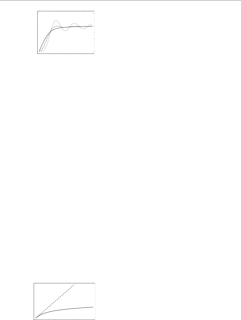
The level number variance
2
(L) is shown to be an
average over the two-level cluster function,
2
ðLÞ¼L 2
Z
L
0
ðL rÞY
2
ðrÞdr ½15
We find L
ffiffiffiffiffiffiffiffiffiffiffiffi
2
(L)
p
levels in an interval of length L.
In the uncorrelated Poisson case, one has
2(P)
(L) = L.
This is just Poisson’s error law. For the Gaussian
ensembles
2()
(L) behaves logarithmically for large L.
The spectrum is said to be more rigid than in the
Poisson case. As Figure 4 shows, the level number
variance probes longer distances in the spectrum, in
contrast to the nearest-neighbor spacing distribution.
Many more observables, also sensitive to higher
order, k > 2 correlations, have been defined. In
practice, however, one is often restricted to analyz-
ing two-level correlations. An exception is, to some
extent, the nearest-neighbor spacing distribution
p(s). It is the two-level correlation function with
the additional requirement that the two levels in
question are adjacent, that is, that there are no levels
between them. Thus, all correlation functions are
needed if one wishes to calculate the exact nearest-
neighbor spacing distribution p
()
(s) for the
Gaussian ensembles. These considerations explain
that we have X
()
2
(s) ’ p
()
(s) for small s. But while
X
()
2
(s) saturates for large s, p
()
(s) quickly goes to
zero in a Gaussian fashion. Thus, although the
nearest-neighbor spacing distribution mathemati-
cally involves all correlations, it makes in practice
only a meaningful statement about the two-level
correlations. Luckily, p
()
(s) differs only very slightly
from the heuristic Wigner surmise [2] (correspond-
ing to = 1), respectively from its extensions
(corresponding to = 2 and = 4).
Ergodicity and Universality
We constructed the correlation functions as averages
over an ensemble of random matrices. But this is not
how we proceeded in the data analysis sketched in
the Introduction. There, we started from one single
spectrum with very many levels and obtained the
statistical observable just by sampling and, if
necessary, smoothing. Do these two averages, the
ensemble average and the spectral average, yield the
same? Indeed, one can show that the answer is
affirmative, if the level number N goes to infinity.
This is referred to as ergodicity in RMT.
Moreover, as already briefly indicated in the
Introduction, very many systems from different
areas of physics are well described by RMT. This
seems to be at odds with the Gaussian assumption
[5]. There is hardly any system whose Hamilton
matrix elements follow a Gaussian probability
density. The solution for this puzzle lies in the
unfolding. Indeed, it has been shown that almost all
functional forms of the probability density P
()
N
(H)
yield the same unfolded corre lation functions, if no
new scale compar able to the mean level spacing is
present in P
()
N
(H). This is the mathematical side of
the empirically found universality.
Ergodicity and universality are of crucial impor-
tance for the applicability of RMT in data analysis.
Wave Functions
By modeling the Hamiltonian of a system with a
random matrix H, we do not only make an
assumption about the statistics of the energies, but
also about those of the wave functions. Because of
the eigenvalue equation Hu
n
= x
n
u
n
, n = 1, ..., N,
the wave function belonging to the eigenenergy x
n
is modeled by the eigenvector u
n
. The columns of
the diagonalizing matrix U = [u
1
u
2
u
N
] are these
eigenvectors. The probability densi ty of the compo-
nents u
nm
of the eigenvector u
n
can be calculated
rather easily. For larg e N it approaches a Gaussian.
This is equivalent to the Porter–Thomas distribu-
tion. While wave functions are often not accessible
in an experiment, one can measure transition
amplitudes and widths, giving information about
the matrix elements of a transition operator and a
0123
r
0.0
0.5
1.0
1.5
X
2
(β
)
(r )
Figure 3 Two-level correlation function X
()
2
(r) for GOE (solid),
GUE (dashed) and GSE (dotted).
0123
L
0
1
2
Σ
2
(L)
Figure 4 Level number variance
2
(L) for GOE (solid) and
Poisson case (dashed).
Random Matrix Theory in Physics 341