Francoise J.-P., Naber G.L., Tsun T.S. (editors) Encyclopedia of Mathematical Physics
Подождите немного. Документ загружается.


large time and large Reynolds number (viscosity
close to 0), the vorticity of the solution of the
Navier–Stokes equations appears in a simple and
organized structure. This stays intact until the
viscous dissipation damps it. The imp ortant obs er-
vation is that the organized structure is described
quite precisely by the solution of the mean-field
equation for some specific .
Actually, to say that a fluid is inviscid is an
approximation (which may be justified in many
contexts), since every fluid displays some kind of
viscosity. But turbulence is a phenomenon occurring
at very small viscosity. In this sense, the above result
provides a description of stationary regime in an
ideal fluid, which is a good approximation of some
numerical simulations of real fluids. Besid es this
good agreement with numerical simulations, there is
no proof on how to deduce the mean-field equation
from the Euler equations (e.g., which parameter
has to be chosen in eqn [38]?).
Remark The extension of this analysis to three-
dimensional flows involves vortex filaments, instead
of point vortices. There are attempts to describe
interacting vortex filaments as proposed by Chorin.
Idealizations of behavior of vortices are introduced
to have a tractable mathematical model. The reader
is referred to Lions (1997) for a description of nearly
parallel vortex filaments and to Flandoli and Bessaih
(2003) for more realistic filaments which fold.
See also: Cauchy Problem for Burgers-Type Equations;
Hamiltonian Fluid Dynamics; Incompressible Euler
Equations: Mathematical Theory; Malliavin Calculus;
Non-Newtonian Fluids; Partial Differential Equations:
Some Examples; Stochastic Differential Equations;
Turbulence Theories; Viscous Incompressible Fluids:
Mathematical Theory; Vortex Dynamics.
Further Reading
Albeverio S and Cruzeiro AB (1990) Global flows with invariant
(Gibbs) measures for Euler and Navier–Stokes two dimensional
fluids. Communications in Mathematical Physics 129: 431–444.
Bensoussan A and Temam R (1973) E
´
quations stochastiques du type
Navier–Stokes. Journal of Functional Analysis 13: 195–222.
Bricmont J, Kupiainen A, and Lefevere R (2001) Ergodicity of the
2D Navier–Stokes equations with random forcing. Commu-
nications in Mathematical Physics 224(1): 65–81.
Da Prato G and Debussche A (2003) Ergodicity for the 3D
stochastic Navier–Stokes equations. Journal de Mathe´ma-
tiques Pures et Applique´es 82(8): 877–947.
E Weinan, Mattingly JC, and Sinai Y (2001) Gibbsian dynamics
and ergodicity for the stochastically forced Navier–Stokes
equation. Communications in Mathematical Physics 224(1):
83–106.
Flandoli F and Bessaih H (2003) A mean field result for 3D vortex
filaments. In: Davies IM, Jacob N, Truman A, Hassan O,
Morgan K, and Weatherill NP (eds.) Probabilistic Methods in
Fluids, 22–34. River Edge, NJ: World Scientific.
Flandoli F and Maslowski B (1995) Ergodicity of the 2-D Navier–
Stokes equation under random perturbations. Communica-
tions in Mathematical Physics 172(1): 119–141.
Frisch U (1995) Turbulence. The legacy of A. N. Kolmogorov.
Cambridge: Cambridge University Press.
Gallavotti G (2002) Foundations of Fluid Dynamics. Berlin:
Springer.
Hairer M and Mattingly JC (2004) Ergodic properties of highly
degenerate 2D stochastic Navier–Stokes equations (English.
English, French summary). Comptes Rendus Mathe´matique.
Acade
´
mie des Sciences. Paris 339(12): 879–888 (see also the
paper ‘‘Ergodicity of the 2D Navier–Stokes equations with
degenerate stochastic forcing’’ to appear on Annals of
Mathematics).
Hopf E (1952) Statistical hydromechanics and functional calculus.
Journal of Rational Mechanics and Analysis 1: 87–123.
Kraichnan RH and Montgomery D (1980) Two–dimensional
turbulence. Reports on Progress in Physics 43(5): 547–619.
Kuksin SB (2004) The Eulerian limit for 2D statistical hydro-
dynamics. Journal of Statistical Physics 115(1/2): 469–492.
Kuksin S and Shirikyan A (2000) Stochastic dissipative PDEs and
Gibbs measures. Communications in Mathematical Physics
213(2): 291–330.
Lions P-L (1997) On Euler Equations and Statistical Physics,
Pubblicazione della Scuola Normale Superiore. Pisa: Cattedra
Galileiana.
Marchioro C and Pulvirenti M (1994) Mathematical Theory of
Incompressible Nonviscous Fluids. Applied Mathematical
Science, vol. 96. New York: Springer.
Mikulevicius R and Rozovskii BL (2004) Stochastic Navier–
Stokes equations for turbulent flows. SIAM Journal on
Mathematical Analysis 35(5): 1250–1310.
Monin AS and Yaglom AM (1987) Statistical Fluid Mechanics:
Mechanics of Turbulence.Cambridge, MA: MIT Press.
Onsager L (1949) Statistical hydrodynamics. Nuovo Cimento
6(suppl. 2): 279–287.
Robert R (2003) Statistical hydrodynamics (Onsager revisited). In:
Friedlander S and Serre D (eds.) Handbook of Mathematical
Fluid Dynamics, vol. II, pp. 1–54. Amsterdam: North-Holland.
Vishik MJ and Fursikov AV (1988)
Mathematical Problems of
Statistical Hydromechanics. Dordrecht: Kluwer Academic
Publishers.
Stochastic Hydrodynamics 79
Stochastic Loewner Evolutions
G F Lawler, Cornell University, Ithaca, NY, USA
ª 2006 Gregory F Lawler. Published by Elsevier Ltd.
All rights reserved.
Introduction
The stochastic Loewner evolution or Schramm–
Loewner evolution (SLE) is a family of random curves
that appear as scaling limits of curves or cluster
boundaries of discrete statistical mechanical models in
two dimensions at criticality. The stochastic Loewner
evolution was introduced by Oded Schramm as a
candidate for the limit of loop-erased random walk
and the boundary of percolation clusters, and it is now
believed that SLE curves appear in most planar critical
systems whose scaling limit satisfies conformal invar-
iance. The curves are defined by solving a Loewner
differential equation with a random input.
Definition
There are three major one-parameter families of SLE
curves – chordal, radial, and whole-plane – which
correspond to curves connecting two boundary points
in a domain, a boundary point and an interior point in
a domain, and two points in C, respectively. The
parameter is usually denoted >0. The starting point
for defining SLE is to write down the assumptions
that one expects from a scaling limit, assuming that
the limit is conformally invariant.
In the chordal case, we assume that there is a
family of probability measures {
D
(z, w)}, indexed
by simply connected proper domains D C and
distinct boundary points z, w 2 @D, supported on
continuous curves : [0, t
] !
D with (0) = z,
(t
) = w, which satisfies the following:
Conformal invariance.Iff : D ! D
0
is a con-
formal transformation, then the image of
D
(z, w)
under f is the same as
D
0
(f (z), f (w)), up to a time
change.
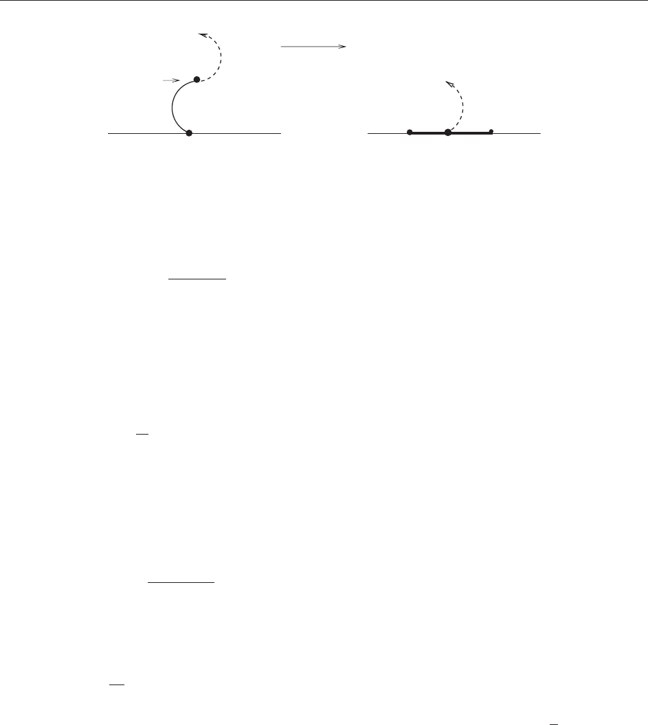
Conformal Markov property for
D
(z, w).
Suppose [0, t] is known, and let g
t
be
a conformal transformation of the slit domain
Dn[0, t] onto D with g
t
((t)) = z, g
t
(w) = w
(see Figure 1). Then the conditional distribution
on g
t
[t, t
], given [0, t], is the same, up to a
change of parametrization, as the original dis-
tribution. (Implicit in this is the assumption that
(t) is on the boundary of Dn(0, t ], which will be
true, e.g., if is non-self-intersecting and
(0, t
) D.)
Using the Riemann mapping theorem, one can see
that such a family {
D
(z, w)} is determined (up
to reparametrization) by
H
(0, 1), where H = {x þ
iy : y > 0} denotes the upper half-plane. Suppose
: [0, 1) ! C is a simple (i.e., no self-intersections)
curve with (0) = 0, (0, 1) H, and sup
t
Im
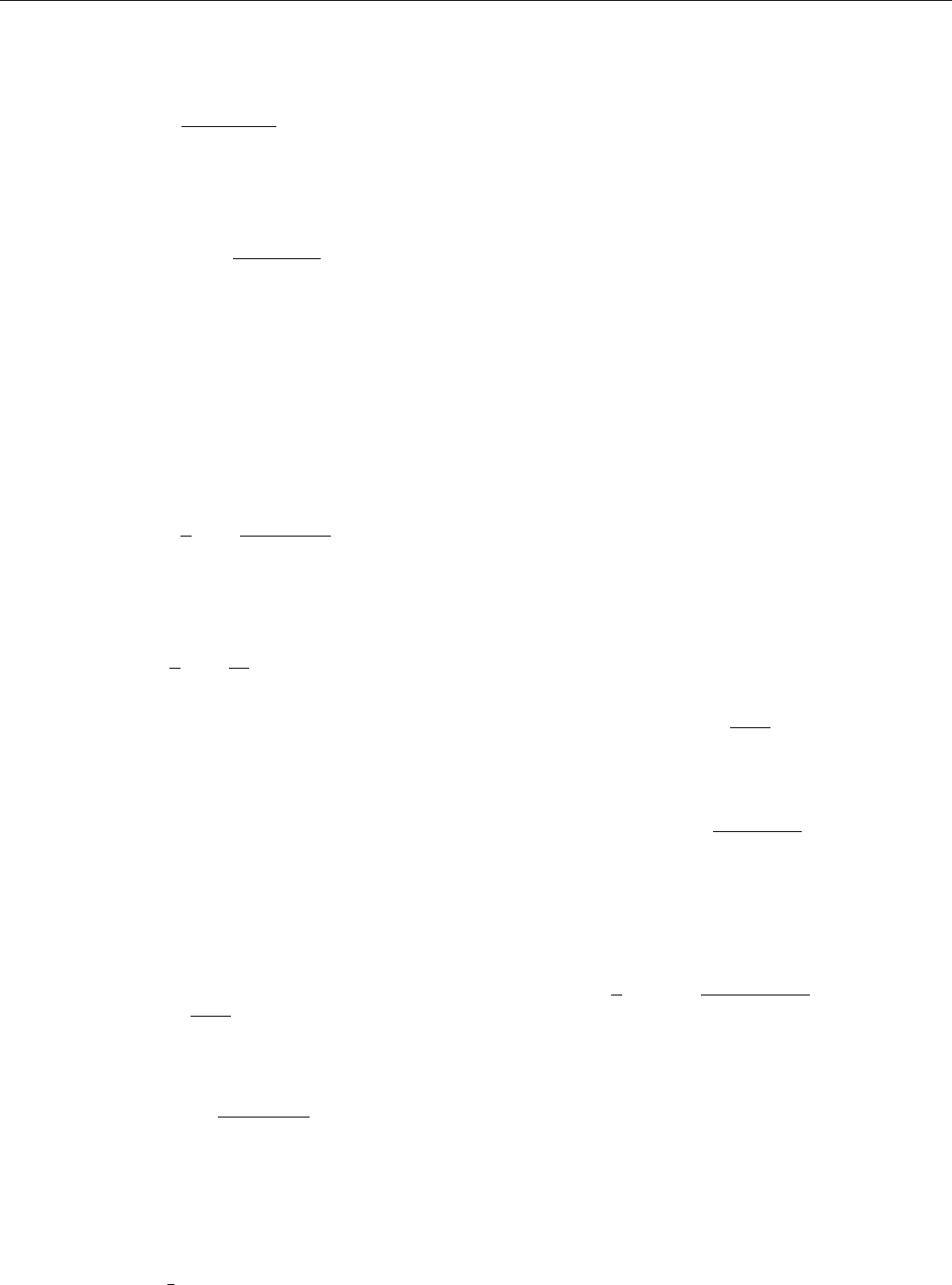
[(t)] = 1. Let H
t
= Hn[0, t]. There is a unique
conformal transformation g
t
: H
t
! H whose
expansion at infinity is
g
t
ðzÞ¼z þ
bðtÞ
z
þ Oðjzj
2
Þ; z !1
(see Figure 2). The coefficient b(t), which is some-
times called the half-plane capacity of [0, t] and
denoted hcap[[0, t]], is continuous, strictly increas-
ing, and tending to 1. In fact,
bðtÞ¼lim
y!1
y E½Im½ X
jX
0
¼ iy
where X
s
denotes a complex Brownian motion and
=
[0, t]
is the first time s such that X
s
2 R [ [0, t].
By reparametrizing , b(t) = 2t. With this parame-
trization, the maps g
t
satisfy the Loewner differen-
tial equation
_
g
t
ðzÞ¼
2
g
t
ðzÞU
t
; g
0
ðzÞ¼z
where U : [0, 1) ! R is a continuous function with
U
0
= 0. In fact, U
t
= g
t
((t)). Schramm observed that
the measure
H
(0, 1), at least if it were supported
on simple curves and the curves were parametrized
using half-plane capacity, would produce a random
U
t
. If the assumptions above on {
D
(z, w)} are
translated into assumptions on the ‘‘driving func-
tion’’ U
t
, one shows readily that U
t
must be a
driftless Brownian motion, that is, U
t
=
ffiffiffi
p
B
t
, for a
standard one-dimensional Brownian motion B
t
.
Chordal SLE
(in H connecting 0 and 1)is
defined to be the random collection of conformal
maps g
t
obtained by solving the initial-value problem
_
g
t
ðzÞ¼
2
g
t
ðzÞ
ffiffiffi
p
B
t
; g
0
ðzÞ¼z ½1
g
t
z
w
w
γ
(t )
z
= g
t
(γ(t))
Figure 1 The map g
t
from D n[0, t] onto D.
80 Stochastic Loewner Evolutions
where B
t
is a standard one-dimensional Brownian
motion. Equation [1] is often given in terms of the
inverse f
t
= g
1
t
:
_
f
t
ðzÞ¼f
0
t
ðzÞ
2
z
ffiffiffi
p
B
t
This equation describes a random evolution of
conformal maps f
t
from H into subdomains of H.
For each z 2
H, the solution of [1] is defined up to a
time T
z
2 [0, 1] with T
z
> 0 for z 6¼ 0. For fixed
t, g
t
is the unique conformal transformation of
H
t
:= {z 2 H : T
z
> t} onto H with expansion
g
t
ðzÞ¼z þ
2t
z
þ; z !1
The chordal SLE
path is the random curve
: [0, 1) ! H such that for each t, H
t
is the
unbounded component of Hn[0, t]. It is not
immediate from the definition that such a curve
exists, but its existence has been proved. If G
t
= g
t=
,
then we can write eqn [1] as
_
G
t
ðzÞ¼
a
G
t
ðzÞþW
t
½2
where a = 2= and W
t
:=
ffiffiffi
p
B
t=
is a standard
Brownian motion. Then Z
z
t
:= G
t
(z) þ W
t
satisfies
the Bessel stochastic differe ntial equation
dZ
z
t
¼
a
Z
z
t
dt þ dW
t
; Z
z
0
¼ z ½3
This equation is valid up to time T
z
, which is the
first time that Z
z
t
= 0.
Although chordal SLE
is defined with a parti-
cular parametrization, one generally thinks of it as a
measure on curves modulo reparametrization. The
scaling properties of Brownian motion imply that
this measure is invariant under dilations of H.IfD
is a simply connected domain and z, w are distinct
boundary points of D, chordal SLE
in D connecting
z and w is defined to be the conformal image of
SLE
in H from 0 to 1 under a conformal
transformation of H onto D taking 0 to z and 1
to w. There is a one-parameter family of such
transformations, but the scale invariance of SLE
in
H shows that the image measure is independent of
the choice of transformation.
The geometric and fractal properties of the curve
vary greatly as the parameter changes:
if 4, is a simple curve;
if 4 <<8, has self-intersections, but is not
space filling; and
if 8, is a space filling curve.
To see this, one notes that the conformal Markov
property implies that there can be double points
with pos itive probability if and only if T
x
< 1
occurs with positive prob ability for x > 0. In add-
ition, the curve is space filling if and only if T
z
< 1
for all z and T
w
6¼ T
z
for w 6¼ z. The problem is then
reduced to a problem about the Bessel equation [3]
for which the following holds:
if a 1 = 2 and z 6¼ 0, the probability that T
z
< 1
is zero. If a < 1=2, this probability equals 1.
if 1=4 < a < 1=2, and w, z are distinct points in H,
then there is a positive probability that T
w
= T
z
.
if 0 < a 1=4, then with probability 1, T
w
6¼ T
z
for all w 6¼ z.
This kind of argument is typical when studying
SLE – geometric properties of the curve are
established by analyzing a stochastic differential
equation. The Hausdorff dimension of the path
is given by
dim½½0; 1Þ ¼ min 1 þ
8
; 2
no
The radial Loewner equation describes the evolu-
tion of a curve from the boundary of the unit disk
D = {z : jzj < 1} to the origin. Suppose : [0, 1) !
D is a simple curve with (0) = 1, (0, 1) Dn{0},
and (t) ! 0ast !1. Let g
t
be the unique
conformal transformation of Dn[0, t] onto D such
that g
t
(0) = 0, g
0
t
(0) > 0. One can check that g
0
t
(0) is
continuous and strictly increasing in t, and hence we
can parametrize in such a way that g
0
t
(0) = e
t
.
Using this reparametrization, there is a continuous
U
0
U
t
g
t
γ (t )
Figure 2 The map g
t
from Hn[0,t] onto H:
Stochastic Loewner Evolutions 81
U
t
: [0, 1) ! R with U
0
= 0 such that g
t
satisfies
the radial Loewner equation
_
g
t
ðzÞ¼g
t
ðzÞ
e
iU
t
þ g
t
ðzÞ
e
iU
t
g
t
ðzÞ
; g
0
ðzÞ¼z
If z 6¼ 0, then we can define h
t
(z) = i log g
t
(z)
locally near z, and this equation becomes
_
h
t
ðzÞ¼cot
h
t
ðzÞU
t
2
Radial SLE
(connecting 1 and 0 in D) is obtained
by setting U
t
=
ffiffiffi
p
B
t
.IfD is a simply connected
domain, z 2 D, w 2 @D, then radial SLE
in D
connecting w and z is obtained by conformal
transformation using the unique transformation
f of D onto D with f (0) = z, f (1) = w. Again, we
think of this as being defined modulo time change. If
a = 2= and v
t
= h
at=2
, then
_
v
t
ðzÞ¼
a
2
cot
v
t
ðzÞþW
t
2
½4
where W
t
:=
ffiffiffi
p
B
t=
is a standard Brownian
motion. If L
z
t
= v
t
(z) þ W
t
, then we get
dL
z
t
¼
a
2
cot
L
z
t
2
dt þ dW
t
Radial and chordal SLE are closely related. In fact, if
is a chordal SLE path in H from 0 to 1,
˜
is a
radial SLE path in D from 1 to 0, and = i log
˜
,
then for small t the distribution of is absolutely
continuous to the distribution of a (random time
change of) . Showing this involves understanding
the behavior of the Loewner equation under
conformal transformations. Suppose ,
˜
have been
parametrized as in [2] and [4] with a = 2=. Let g
t
be the conformal transformation of Hn[0, t] onto
H such that
g
t
ðzÞ¼z þ
a
ðtÞ
z
þ; z !1
and let U
t
be the Loewner driving function such that
_
g
t
ðzÞ¼
_
a
ðtÞ
g
t
ðzÞU
t
Here a
(t) = hcap[[0, t]]. If we consider a time
change such that a
((t)) = at and let U
t
=
~
U
(t)
be the time-changed driving function, Itoˆ ’s formula
can be used to show that
dU
t
¼
1
2
ð1 3aÞF
t
dt þ d
~
W
t
½5
where the F
t
in the drift term depends on [0, t] and
is independent of a, and
~
W is a standard Brownian
motion. Girsanov’s theorem implies that Brownian
motions with the same variance but different drifts
have ab solutely continuous distributions. In parti-
cular, qualitative properties such as existence of
double points or Hausdorff dimension of paths are
the same for radial and chordal SLE. U
t
is a driftless
Brownian motion if a = 1=3, = 6.
Whole-plane SLE
from 0 to 1 is a p ath
:(1, 1) ! C with (1) = 0, (1) = 1,such
that gi ven (1, t], the distribution of (t, 1)is
that of radial SLE
from boundary point (t)to
interior point 1 in the domain Cn[1, t]. One can
define whole-plane SLE
connecting two distinct
points in C by confor mal transformat ion.
Locality and Restriction
There are two special values of : = 6, a = 1= 3that
satisfies the ‘‘locality’’ property and = 8 = 3, a = 3=4
that satisfies the ‘‘restriction’’ property. Suppose is a
chordal SLE
curve from 0 to 1 in H parametrized
as in [2].Suppose : N!H is a conformal map
taking a neighborhood N of 0 in H to (N) and that
locally maps R into R.Let
˜
(t) = (t), which is
defined for sufficiently small t.Letg
t
be the
conformal transformation of Hn
˜
[0, t] onto H with
g
t
ðzÞ¼z þ
a
ðtÞ
z
þ
and let
~
U
t
be the driving function such that
_
g
t
ðzÞ¼
_
a
ðtÞ
g
t
ðzÞ
~
U
t
Here a
(t) = hcap[
˜
[0, t]]. If we change time,
t
=
~
(t)
, so that a
((t)) = at, then an application
of Itoˆ ’s formula shows that U
t
:=
~
U
(t)
satisfies
dU
t
¼
1
2
ð3a 1Þ
00
ðtÞ
ðW
ðtÞ
Þ
0
ðtÞ
ðW
ðtÞ
Þ
2
dt þ d
~
W
t
Here
~
W
t
is a standard Brownian motion,
t
= g
t
g
1
t
, and g
t
is the conformal map associated to .
In particular, if a = 1=3, = 6, U
t
is a standard
Brownian motion; hence,
~
has the distribution of
SLE
6
. The locality property for SLE
6
can be stated
as ‘‘the conformal image of SLE
6
is (a time change
of) SLE
6
.’’ Intuitively, the SLE
6
path in a restricted
domain does not feel the boundary of the domain
until it reaches it. Radial SLE
6
satisfies a similar
locality property. Moreover, [5] can be used to
show that the image of chordal SLE
6
under the
exponential map is the same (for small time t)as
radial SLE
6
. The locality property explains why
82 Stochastic Loewner Evolutions

SLE
6
is a natural candidate for the boundary of
percolation clusters.
If 4, SLE
paths are simple, that is, with no
self-intersections. Suppose A
Hn{0} is a compact
set such that HnA is simply connected. Let denote
a chordal SLE
in H connecting 0 and 1 and
let E
A
be the event E
A
= {(0, 1) \ A = ;}. Let
A
: HnA ! H be the unique conformal transforma-
tion with
A
(0) = 0,
A
(1) = 1,
0
A
(1) = 1. On
the event E
A
, we can define
˜
(t) =
A
(t). Chorda l
SLE
is said to satisfy the restriction property if the
conditional distribution of
˜
given E
A
is the same as
(a time change of) . The only 4 that satisfies
this property is = 8=3. The proof of this fact also
establishes the formula: if is a chordal SLE
8=3
curve in H from 0 to 1, then
Pfð0; 1Þ \ A ¼;g¼
0
A
ð0Þ
5=8
½6
There is a similar formula for radial SLE
8=3
, which
establishes a radial restriction property. Suppose
A
Dn{0, 1} is a compact set such that DnA is
simply connected. Let
A
be the unique conformal
transformation of DnA onto D with
A
(0),
0
A
(0) > 0.
Then, if is a radial SLE
8=3
curve from 1 to 0 in D,
then
Pfð0; 1Þ \ A ¼;g¼
0
A
ð0Þ
5=48
j
0
A
ð1Þj
5=8
The restriction property makes SLE
8=3
the candidate
for the scaling limit of self-avoiding walks.
Relation to Conformal Field Theory
The Schramm–Loewner evolution is one of the tools
used to rigorously prove predictions made using
powerful, yet nonrigorous, arguments of conformal
field theory. In conformal field theory, there is a
parameter c, called the central charge, which
classifies theories. To each c 1, there corresp onds
a 4 and a ‘‘dual’’
0
= 16= 4:
c ¼ c
¼
ð8 3Þð 6Þ
2
In particu lar, = 8=3,
0
= 6 corresponds to central
charge zero. It is expected, and has been proved in a
number of cases, that SLE
or SLE
0
curves will
appear in scaling limits of systems with central
charge c
. These systems can also be param etrized
by the boundary scaling exponent or conformal
weight
¼
¼
6
2
For = 8=3, = 5=8 which is the exponent in [6].
In studying the relationship between SLE and
conformal field theories, two other probabilistic
objects, restriction measures and the (Brownian)
loop soup, arise. An H-hull (connecting 0 and 1 )is
an unbounded, connected, closed set K
H with
K \ R = {0} and such that HnK consists of two
connected components, one whose boundary
includes the positive reals and the other whose
boundary includes the negative reals. A (chordal)
restriction measure on hulls K is a probability
measure with the property that for any A as in [6],
the distribution of
A
K given {K \ A = ;} is the
same as the original measure. The (Brownian) loop
measure is a measure on unrooted loops derived
from Brownian bridges. It is the scaling limit of the
measure on random walk loops that gives each
unrooted simple random walk loop of length 2n
measure 4
2n
. The loop measure in a bounded
domain is obtained by restricting to loops that stay
in that domain. We can consider this as a measure
on ‘‘hulls’’ by fill ing in the bounded holes (so that
the complement of the hull is connected). By doing
this we get a family of infinite measures on hulls,
indexed by domains D, and this family satisfies
conformal invariance and the restriction property.
The loop soup with parameter is a Poissonian
realization from this measure with parameter .
The set of all restriction measures is parametrized
by 5=8; the -restriction measure has the
property that
PfK \ A 6¼;g¼
0
A
ð0Þ
For = 5=8, K is given by the path of SLE
8=3
. For
integer , the hull K can be constructed by taking
-independent Brownian excursions in H (Brownian
motions starting at 0 conditioned to stay in H for all
times), and letting K be the hull obtain ed by taking
the union of the paths and filling in the bounded
holes. If 8=3, c
0, then the restriction mea-
sure with exponent
5=8 can also be con-
structed as follows: take a chordal SLE
path and
an independent realization of the loop soup with
intensity
= c
; add to the SLE path all the
loops in the soup that intersect the SLE
curve; and
then fill in all the bounded hulls. The limiting case
= 5=8, = 0 gives the only measure supported on
simple curves that is also a restriction measure,
SLE
8=3
.
For 8=3 < 4, 0 < c
1, it is conjectured,
and proved for small c
, that SLE
curves can be
found by taking a loop soup with parameter = c
and looking at connected curves in the fractal set
given by the complement of the union of all the hulls
generated by the loops.
Stochastic Loewner Evolutions 83
Examples
The scaling limit of simple random walk, Brownian
motion, is known to be conformally invariant. A
two-dimensional Brownian bridge or loop is a
Brownian motion, B
t
,0 t 1, conditioned so
that B
0
= B
1
. The frontier or outer boundary of the
Brownian motion is the boundary of the unbounded
component of the complement. Benoit Mandelbrot
first observed numerically that the outer boundary
of Bro wnian motion had fractal dimensi on 4=3.
Gregory Lawler, Oded Schramm, and Wendelin
Werner used SLE to prove that the boundary has
Hausdorff dimension 4/3. In fact, the outer bound-
ary can be considered as an SLE
8=3
loop.
SLE
6
and SLE
8=3
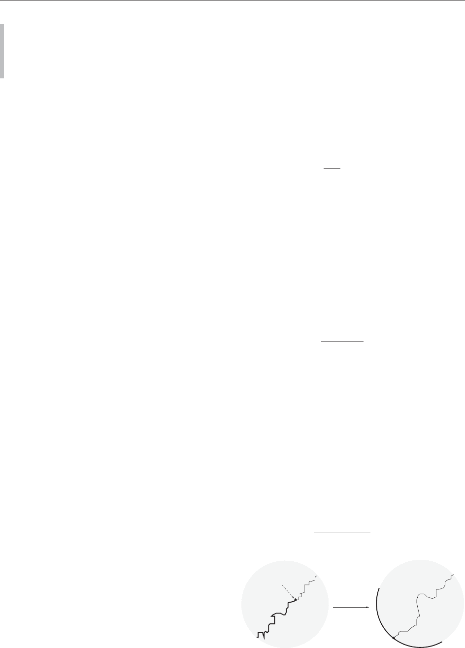
arise in the scaling limit of
critical percolation on the triangular lattice. Suppose
that each vertex in the upper half-plane triangular
lattice is colored black or white each with a
probability 1/2. Suppose the real line gives a
boundary condition of black on the negative real
line and white on the positive real line. Then if we
represent the vertices in the lattice as hexagons as
in the figure, a curve is formed which is the
boundary between the black and white clusters.
This curve is called the ‘‘percolation exploration
process.’’ Stanislav Smirnov proved that the scaling
limit of this curve is conformally invariant, and from
this it can be concluded that the curve is chordal
SLE
6
. In particular, the Hausdorff dimension is 7/4
and the scaling limit has double points. In the
scaling limit, the ‘‘outer boundary’’ of this curve has
Hausdorff dimension 4/3 and its dimension is
absolutely continuous with respect to that of
SLE
8=3
. While this result is expected for other
critical percolation model, such as bond percolati on
in Z
2
with critical probability 1/2, it has only been
proved for the triangular lattice. Percolation has
central charge 0 and the ‘‘locality’’ propert y can be
seen in the lattice model. The outer boundary of the
curve has the same distribution as the outer
boundary of a Brownian motion that is reflected at
angle =3 off the real line. Locally, the outer
boundary of percolation, the outer boundary of
complex Brownian motion, and SLE
8=3
all look the
same, and it is expected that this will also be true for
the scaling limit of self-avoiding walks.
There are three models derived in some way from
simple random walk that have been proved to have
scaling limits of SLE
. The loop-erased random walk
(LERW) in a finite subset V of Z
2
connecting two
distinct points is obtained by taking a simple
random walk from one point to the other and
erasing loops chronologically. The LERW is closely
related to uniform spanning trees; in fact, if one
chooses a spanning tree of V from the uniform
distribution on all spanning trees, then the distribu-
tion of the unique path connecting the two points is
exactly that of the LERW (see Figure 3). Another
description of the LERW is as the Laplacian random
walk: the LERW from z to w in V chooses a new
step weighted by the value of the function that is
harmonic on the complement of w and the path up
to that point with boundary values 0 on the path
and 1 on w. The LERW in the discrete upper half-
plane can be obtained by erasing loops from a
simple random walk excursion. The LERW and the
uniform spanning tree are systems with central
charge c = 2. It has been proved that the scaling
limit of the LERW is SLE
2
; hence, the paths have
Hausdorff dimension 5/8.
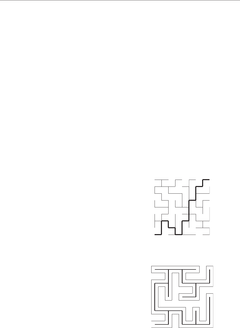
There is another path associated to spanning trees
given by the one-to-one correspondence between
spanning trees and Hamiltonian walks on a corre-
sponding directed (Manhattan) lattice on the dual
graph (see Figure 4). If the spanning trees, or
equivalently the Hamiltonian walks, are chosen
using the uniform distribution, then the scaling
limit of this walk is the space-filling curve SLE
8
.
Note that 2 and 8 are the dual values of associated
to c = 2.
Figure 3 A spanning tree and the path between two vertices.
If the tree has the uniform distribution, the path has the
distribution of the LERW.
Figure 4 A spanning tree and the corresponding Hamiltonian
walk.
84 Stochastic Loewner Evolutions

Another discrete process derived from simple
random walk, the harmonic explorer, has a scaling
limit of SLE
4
. There is a particular property of SLE
that leads to the definition of this discrete process.
Consider a chordal SLE
curve, let z 2 H, and let Z
z
t
be as in [3] with a = 2= . Itoˆ ’s formula shows that
t
:= arg(Z
z
t
) satisfies
d
t
¼
1
2
a
sinð2
t
Þ
jZ
z
t
j
2
dt
sin
t
jZ
z
t
j
dW
t
In particular,
t
is a martingale if and only if
a = 1=2, = 4. The probability that a complex
Brownian motion starting at z 2 H first hits R on
the negative half-line can be sh own to be arg (z). If
4, then we can see that
1
equals 0 or ,
depending on whether z is on the right or left side
of the path (0, 1). For the martingale case = 4,
t
represents the probability that z is on the left
side of (0, 1), given (0, t]. The harmonic
explorer is a pro cess on the hexagonal lattice
defined to have this property. In a way similar to
the percolation process, the walk is defined as the
boundary between black and white hexagons on
the triangular lattice. However, when an unex-
plored hexagon is reached in the harmonic
explorer, it is colored black with probability q,
where q is the probability that a simple random
walk on the triangular lattice starting at that
hexagon (considered as a vertex in the triangular
lattice) hits a black hexagon before hitting a white
hexagon. It is not difficult to show that this process
has the property that for z away from the curve,
the ‘‘probability of z ending on the left given the
curve of n steps’’ is a martingale.
There are many other models for which SLE
curves are expected in the limit, but it has not been
established. The most difficult part is to show the
existence of a limit that is conformally invariant.
One example is the self-avoiding walk (SAW). It is
an open problem to establish that there exists a
scaling limit of the uniform measure on SAWs and
to establish conformal invariance of the limit.
However, the nature of the discrete model is such
that if the limit exists, it must satisfy the restriction
property. Hence, under the assumption of confor-
mal invariance, the only possible limit is SLE
8=3
.
Numerical simulations strongly support the con-
jecture that SLE
8=3
is the limit of SAWs, and this
gives strong evidence for the conformal invariance
conjecture for SAWs. Critical exponents for SAWs
(as well as critical exponents for many other
models) can be predicted nonrigorously from
rigorous scaling exponents for the corresponding
SLE paths.
Generalizations
One of the reasons that the theory of SLE is nice for
simply connected domains is that a simply connected
domain with an arc connected to the boundary of the
domain removed is again simply connected. For
nonsimply connected domains, it is more difficult to
describe because the conformal type of the slit
domain changes as time evolves. In the case of a
curve crossing an annulus, this can be done with an
added parameter referring to the conformal type of
the annulus (two annuli of the form {z : r
j
< jzj < s
j
}
are conformally equivalent if and only if
r
1
=s
1
= r
2
=s
2
). It is not immediately obvious what
the correct definition of SLE should be in general
domains and, more generally, on Riemann surfaces.
One possibility for 4 is to consider a configura-
tional (equilibrium statistical mechanics) view of
SLE. Consider a family of measures {
D
(z, w)},
where D ranges over domains and z, w are distinct
boundary points at @D is locally analytic, supported
on simple curves from z to w (modulo time change).
Let
#
D
(z, w) =
D
(z, w)= j
D
(z, w)j be the correspond-
ing probability measures, which may be defined even
if @D is not smooth at z, w. Then the following
axioms should hold:
Conformal invariance.Iff : D ! D
0
is a confor-
mal transformation, f
#
D
(z, w) =
#
D
0
(f (z), f (w)).
Conformal Markov property.
Perturbation of domains. Suppose D
1
D and
@D
1
, @D agree near z, w. Then
D
1
(z, w) should
be absolutely continuous with respect to
D
(z, w).
Let Y denote the Radon–Nikodym derivative of
D
1
(z, w) with respect to
D
(z, w). Then
YðÞ¼1fð 0; t
ÞD
1
g F
c
ðD; ; DnD
1
Þ
where F
c
is to be determined. In the case where
D, D
1
are simply connected, F
c
(D; , DnD
1
) =
J(, D, D
1
)
c
, where J(, D, D
1
) denotes the prob-
ability that there is a loop in the Brownian loop
soup in D that intersects both and DnD
1
. (There
is no problem defining this quantity in nonsimply
connected domains, but it is not clear that it is the
right quantity.) Here c = c
. The restriction property
tells us that F
0
1.
Conformal covariance.Iff is as above, @D, @D
0
are
smooth near z, w and f (z), f (w), respectively, then
f
D
ðz; wÞ¼jf
0
ðzÞj
jf
0
ðwÞj
D
0
ðf ðzÞ; f ðwÞÞ
Here =
is the boundary scaling exponent.
See also: Boundary Conformal Field Theory; Percolation
Theory; Random Walks in Random Environments.
Stochastic Loewner Evolutions 85

Further Reading
Kager W and Nienhuis B (2004) A guide to stochastic Loewner
evolution and its applications. Journal of Statistical Physics
115: 1149–1229.
Lawler G (2004) Conformally invariant processes in the plane. In:
School and Conference on Probability Theory, ICTP Lecture
Notes, vol. 17, pp. 305–351. Trieste, Italy: ICTP.
Lawler G (2005) Conformally Invariant Processes in the Plane.
Providence, RI: American Mathematical Society.
Lawler G and Werner W (2004) The Brownian loop soup.
Probability Theory Related Fields 128: 565–588.
Lawler G, Schramm O, and Werner W (2004a) Conformal
restriction, the chordal case. The Journal of American
Mathematical Society 16: 917–955.
Lawler G, Schramm O, and Werner W (2004b) Conformal
invariance of planar loop-erased random walks and uniform
spanning trees. Annals of Probability 32: 939–995.
Schramm O (2000) Scaling limits of loop-erased random walks
and uniform spanning trees. Israel Journal of Mathematics
118: 221–288.
Smirnov S (2001) Critical percolation in the plane: conformal
invariance, Cardy’s formula, scaling limits. Comptes rendus
de l’Academie des sciences – series i – mathematics 333:
239–244.
Werner W (2003) SLEs as boundaries of clusters of Brownian
loops. Comptes rendus de l’Academie des sciences – series i –
mathematics 337: 481–486.
Werner W (2004) Random planar curves and Schramm–Loewner
evolutions. In: Ecole d’Ete´ de Probabilite´s de Saint-Flour
XXXII – 2002, Lecture Notes in Mathematics, vol. 1840,
pp. 113–195. Berlin: Springer.
Stochastic Resonance
S Herrmann, Universite
´
Henri Poincare
´
, Nancy 1
Vandoeuvre-le
`
s-Nancy, France
P Imkeller, Humboldt Universita
¨
t zu Berlin,
Berlin, Germany
ª 2006 Elsevier Ltd. All rights reserved.
Introduction
The concept of stochastic resonance was introduced
by physicists. It originated in a toy model designed
for a qualitat ive description of periodicity phenom-
ena in the recurrences of glacial eras in Earth’s
history. It spread its popularity over numerous areas
of natural sciences: neu ronal response to periodic
stimuli, variations of magnetization in a ferromag-
netic system, voltage variations in the simple Schmitt
trigger electronic circuit or in more complicated
devices, behavior of lasers in optical bi-stability, etc.
The interest in this ubiquitous phenomenon is
enhanced by signal analysis: an optimal dose of
noise in some system can essentially boost signal
transduction. Noise in this context does not enter the
system as an impurity perturbing its performance, but
on the contrary as a catalyst triggering amplified
stochastic response to weak periodic signals.
The Climate Paradigm
The phenomenon of stochastic resonance was first
discovered in an elementary climate model serving in
an explanation of major transitions in paleoclimatic
time series confining glacial cycles. Data collected
for instance from ice or deep sea cores allow one to
deduce estimates of the average temperature on
Earth over the last 700 000 years. They exhibit
periodic switching between ice and warm ages with
fast spontaneous transitions. The averag e periodicity
of the glaciation time series obtained is 10
5
years.
In order to explain temperature variations, Ben zi
et al. (1981) introduced random perturbations into
an energy balance model of the Budyko–Sellers type.
This model describes the evolution of the seasonal
and global average temperature X caused by defects
in the balance between incoming and outgoing
radiation
c
dXðtÞ
dt
¼E
in
E
out
where c is the active thermal inertia of the system.
The incoming energy is modeled as proportional
to the ‘‘solar constant’’ Q:
E
in
¼ Q 1 þ A cos
2t
T
; with T 92 000 years
and A 0.1% of Q. This exceedingly small varia-
tion of the solar constant is caused by a mod ulation
of the orbital eccentricity of the Earth’s trajectory
(Figure 1). The outgoing radiation E
out
is composed
Figure 1 Modulation of the orbital eccentricity.
86 Stochastic Resonance
of two essential parts. The first part a(X)E
in
is
dominated by the albedo a(X) representing the
proportion of energy reflected back to space. It is a
decreasing function of temperature, due to the
higher rate of reflection from a brighter Earth at
low temperatures implying a bigger volume of ice.
The second part of the outgoing radiation comes
from the fact that the Earth radiates energy like a
black body, and is given by the Boltzmann law X
4
,
where is the Stefan constant. Describing the
balance of energy terms as a slowly and weakly
time-varying gradient of a potential U, the balance
model can be expressed by
dXðtÞ
dt
¼
@U
@x
t
T
; XðtÞ
where the time period 1 is blown up to (large) T by
time scaling. The roles of deep and shallow wells
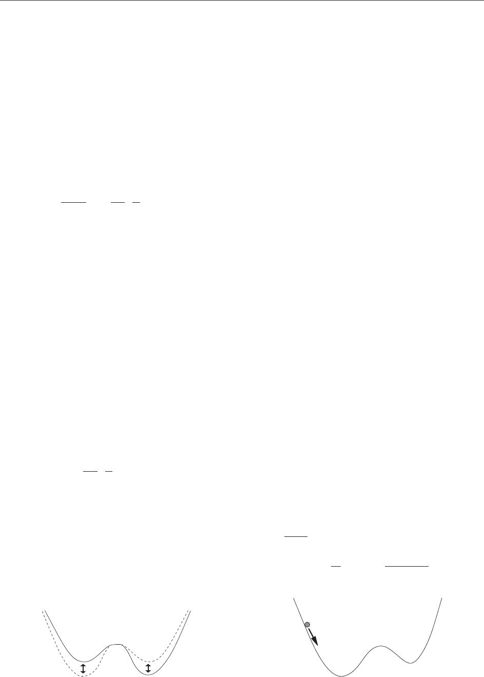
switch periodically (Figure 2). Since the variation of
the solar constant is extremely small, we can assume
that the height of the barrier between the two wells
is lower-bounded by a positive constant. The system
then admits three steady states two of which are
stable and separated by roughly 10 K. As the solar
constant, they fluctuate slowly and very weakly.
Therefore, this deterministic system cannot account
for climate changes with temperature variations of
10 K. They can only be explained by allowing
transitions between the two steady states which
become possible by adding noise to the system. In
general, short timescale phenomena such as annual
fluctuations in solar radiation are modeled by
Gaussian white noise of intensity " and lead to
equations of the type
dX
"
t
¼
@U
@x
t
T
; X
"
t
dt þ
ffiffiffi
"
p
dW
t
½1
which are generic for studying stochastic resonance
in numerous physical and biological models. Gen-
erally, the input of noise amplifies a weak periodic
signal by creating trajectories fluctuating randomly
periodically between meta-stable states. An optimal
tuning of noise intensity to peri od length (‘‘stochas-
tic resonance’’) significantly enhances the response
of the random system to weak perturbations with
long periods.
Strongly Damped Brownian Particle
It is useful to roughly compare solutions of
stochastic differential equations and motions of
Brownian particles in double-well landscapes
(Figure 3) in order to understand properties of
their trajectories (see Schweitzer 2003, Mazo 2002).
As in the previou s section, let us concentrate on a
one-dimensional setting, remarki ng that we shall
give a treatment that easily generalizes to the finite-
dimensional setting. Due to Newton’s law, the
motion of a parti cle is governe d by the impact of
all forces acting on it. Let us denote F the sum of
these forces, m the mass, x the space coordinate, and
v the velocity of the particle. Then
m
_
v ¼F
Let us first assume the poten tial to be switched off.
In their pioneering work at the turn of the
twentieth century, Marian v. Smoluchowski and
Paul Langevin introduced stochastic concepts to
describe the Brownian particle motion by claiming
that at time t
FðtÞ¼
0
vðtÞþ
ffiffiffiffiffiffiffiffiffiffiffiffiffiffiffiffi
2k
B
T
0
p
_
W
t
The first term results from friction
0
and is velocity
dependent. An additional stochastic force represents
random interactions between Brownian particles and
their simple molecular random environment. The
white noise
_
W (formal derivative of the Wiener
process) plays the crucial role. The diffusion coefficient
(standard deviation of the random impact) is com-
posed of Boltzmann’s constant k
B
, friction, and
environmental temperature T. It satisfies the condition
of the fluctuation–dissipation theorem expressing the
balance of energy loss due to friction and energy gain
resulting from noise. The equation of motion becomes
dxðtÞ
dt
¼vðtÞ
dvðtÞ¼
0
m
vðtÞdt þ
ffiffiffiffiffiffiffiffiffiffiffiffiffiffiffiffi
2k
B
T
0
p
m
dW
t
Figure 2 Deep and shallow wells switching periodically.
Figure 3 Brownian particle in a double-well landscape.
Stochastic Resonance 87
In the stationary regime, the stationary Ornstein–
Uhlenbeck process provides its solution
vðtÞ¼v ð0Þe
ð
0
=mÞt
þ
ffiffiffiffiffiffiffiffiffiffiffiffiffiffiffiffi
2k
B
T
0
p
m
Z
t
0
e
ð
0
=mÞðtsÞ
dW
s
The ratio :=
0
=m determines the dynamic behav-
ior. Let us focus on the over-damped situation with
large friction and very small mass. Then for
t >>1= = (relaxation time), the first term in the
expression for velocity can be neglected, while the
stochastic integral represents a Gaussian process. By
integrating, we obtain in the over-damped limit
( !1) that v and thus x is Gaussian with almost
constant mean
mðt Þ¼xð0Þþ
1 e
t
vð0Þxð0Þ
and covariance close to the covariance of white
noise see Nelson (1967):
Kðs; tÞ¼
2k
B
T
0
minðs; tÞþ
k
B
T
0
ð2 þ2e
t
þ2e
s
e
jtsj
e
ðt þsÞ
Þ
2k
B
T
0
minðs; tÞ
Hence, the time-dependent change of the velocity of
the Brownian particle can be neglected, the velocity
rapidly thermalizes (
_
v 0), while the spactial coor-
dinate remains far from equilibrium. In the so-called
adiabatic transformation, the evolution of the
particle’s position is thus given by the transformed
Langevin equation
dxðtÞ¼
ffiffiffiffiffiffiffiffiffiffiffiffi
2k
B
T
p
0
dW
t
Let us next suppose that we have a Brownian
particle in an external field of force (see Figure 3),
generating a potential U(t, x). This leads to the
Langevin equation
dxðtÞ
dt
¼vðtÞ
m dvðtÞ¼
0
vðtÞdt
@U
@x
ðt; xðtÞÞþ
ffiffiffiffiffiffiffiffiffiffiffiffiffiffiffiffi
2k
B
T
0
p
dW
t
In the over-damped limit, after relaxation time, the
adiabatic elimination of the fast variables (Gardiner
2004) leads to an equation similar to the one
encountered in the previous section:
dxðtÞ¼
1
0
@U
@x
ðt; xðtÞÞ þ
ffiffiffiffiffiffiffiffiffiffiffiffi
2k
B
T
p
0
dW
t
In the particular case of some double-well potential
x !U(t, x) with slow periodic variation, the follow-
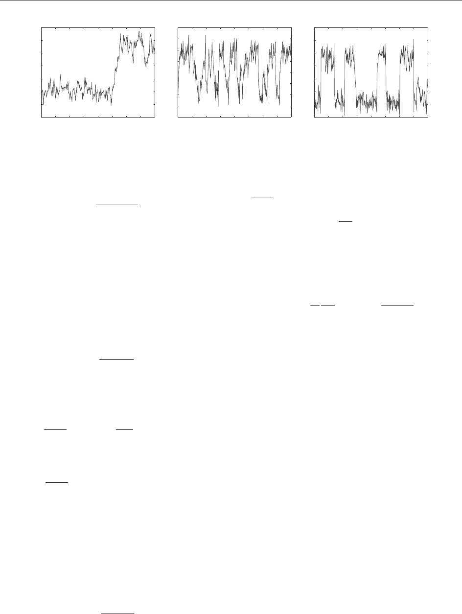
ing patterns of behavior of the solution trajectories
will be experienced. If temperature is high, noise has
a predominant influence on the motion, and the
particle often crosses the barrier separating the two
wells during one period. The behavior of the particle
does not seem to be periodic but rather chaotic. If
temperature is small, the particle stays for a very
long time in the starting well, fluctuating weakly
around the equilibrium position. It has too low
energy to follow the periodic variation of the
potential. So in this case too, the traject ories do
not look periodic. Between these two extreme
situations, there exists a regime of noise intensities
for which the energy transmitted by the noise is
sufficient to cross the barrier almost twice per
period. The parameters are then near to the
resonance point and the motion exhibits periodic
switching (Figure 4).
Transition Criteria
and Quasideterministic Motion
Studying stochastic resonance accordingly means
looking for the range of regimes for which periodic
behavior is enhanced and eventually optimal. The
optimal relation between period T and noise
0 T 2T 3T 4T
–2
–1
0
1
–2
–1
0
1
0 T 2T 3T 4T
2
0 T 2T 3T 4T
–1
0
1
2
Figure 4 Resonance pictures for diffusions.
88 Stochastic Resonance