Francoise J.-P., Naber G.L., Tsun T.S. (editors) Encyclopedia of Mathematical Physics

Подождите немного. Документ загружается.

Supermanifolds

F A Rogers, King’s College London, London, UK

Introduction

A supermanifold is a generalization of a classical

manifold to include coordinates that are in some

sense anticommuting. Much of the motivation for

the study of supermanifolds comes from super-

symmetric physics, where it is useful to have a

formalism which treats fermions and bosons in the

same way. The underlying reason for the effective-

ness of supermanifolds is that anticommuting

coordinates allow the fermionic canonical anti-

commutation relations to be handled in a way

analogous to the bosonic canonical commutation

relations. Supersymmetric methods have proved

immensely effective in fundamental physics; they

also play a considerable role in geometrical index

theory in mathematics. In this article we describe

supermanifolds from two points of view – geometric

and algebraic – and consider some of the standard

features of manifold calculus, including integration

since this is an area where the distinctive features of

this generalized geometry are particularly apparent.

One situation where supermanifolds are used in

physics is in the superspace formulation of super-

gravity, where the physical fields are found in the

component fields in the Taylor expansion of func-

tions on the supermanifold in anticommuting vari-

ables. More fundamentally, the symmetry groups of

supersymmetric theories have commuting and anti-

commuting generators, and are examples of super Lie

groups, which are supermanifolds with a compatible

group structure.

Some Algebraic Preliminaries

The coordinates of a supermanifold have particular

algebraic features which are best understood by

introducing some of the basic concepts of super-

algebra. (The word super here does not imply

superiority, simply the extension of some classical

concept to have odd as well as even, anticommuting

as well as commuting, elements.) A ‘‘super vector

space’’ is a vector space V together with a direct sum

decomposition

V ¼ V

 V

½1

The subspaces V

and V

are referred to, respec-

tively, as the even and odd parts of V. A general

element v of V thus has the unique decomposition

v = v

þ v

with v

in V

and v

in V

. We will

normally consider homogeneous elements, that is,

elements v which are either even or odd, with parity

denoted by jvj, so that jvj= i if v is in V

, i = 0, 1.

(Arithmetic of parity indices i = 0, 1 is always

modulo 2.) A superalgebra is a super vector space

whose elements can be multiplied together in such a

way that the product of an even element with an

even element and that of an odd element with an

odd element are both even, while the product of an

odd element with an even element is odd; more

formally:

Definition 1

130 Supermanifolds

(128)

(i) A ‘‘superalgebra’’ is a super vector space

A = A

 A

which is also an algebra which

satisfies A

 A

iþj

(ii) The superalgebra is ‘‘supercommutative’’ if, for

all homogeneous a, b in A, ab = (1)

(jajjbj)

ba.

If the algebra is supercommutative then odd

elements anticommute, and the square of an odd

element is zero. The basic supercommutative super-

algebra used is the real Grassmann algebra with

generators 1, 

, 

, ... and relations

1

¼ 

1 ¼ 

;



¼



½2

A typical element of this algebra is then

a ¼ a

;

1 þ



i<j



 ½3

This algebra, which is denoted R

, is a superalgebra

with R

:= R

S,0

 R

S,1

, where R

S,0

consists of linear

combinations of products of even numbers of the

anticommuting generators, while R

S,1

is built simi-

larly from odd products.

The Grassmann algebra R

is used to build the

(m, n)-dimensional superspace R

m,n

in the following

way:

Definition 2. An (m, n)-dimensional superspace is

the space

m;n

¼ R

R

|ﬄﬄﬄﬄﬄﬄﬄﬄﬄﬄﬄﬄ{zﬄﬄﬄﬄﬄﬄﬄﬄﬄﬄﬄﬄ}

m copies

R

R

|ﬄﬄﬄﬄﬄﬄﬄﬄﬄﬄﬄﬄ{zﬄﬄﬄﬄﬄﬄﬄﬄﬄﬄﬄﬄ}

n copies

½4

A typical element of R

m, n

is written as

, ..., x

; 

, ..., 

), where the convention is

used that lower case Latin letters represent even

objects and lower case Greek letters represent odd

objects, while small capitals are used for objects of

mixed or unspecified parity.

As will be described in more detail below, in the

geometric approach supermanifolds are spaces

locally modeled on R

m,n

. In order to define a

supermanifold, we will need to define a topology

on this space, and to have some notion of

differentiation. Consider first multilinear functions

of purely anticommuting variables. If there are n

such variables, 

, ..., 

, then a multilinear function

F can be expressed in the form

Fð

; ...;

Þ¼F

;

i¼1



1¼i<j



þ

1...n



...

½5

where the coefficients

;

, F

and so on are real

numbers. Such functions will be known (anticipating

the terminology for functions of both odd and even

variables) as supersmooth. (A useful notation will be

to write

Fð

; ...;

Þ¼







½6

with  a multi-index  = 



and 











1. The set of multi-indices is restricted to

those where 1  

< <

 n.) More general

supersmooth functions, with the coefficients

;

, ...

taking values in C, R

, or some other algebra are

also possible.

Differentiation of supersmooth functions of anti-

commuting variables is defined by linearity together

with the rule

@ð







...



@

ð1Þ

k1





...





...



if j ¼ 

0 otherwise



½7

where the caret bindicates an omitted factor.

In order to extend the notion of supersmoothness

to functions on the more general superspace R

m,n

we should strictly take note of the fact that an even

Grassmann variable is not simply a real or complex

variable, as explained in the appendix. Assuming

this done, a supersmooth function on the general

superspace R

m, n

can then be defined as a function of

the form

Fðx

; ...; x

;

; ...;

Þ¼



ðx

; ...; x

Þ



½8

with each coefficient function



a smooth function

on R

The final preparatory idea needed is the topology

on the superspace R

m, n

. It turns out that a coarse,

non-Hausdorff topology leads to most of the super-

manifolds used in physics. In order to define this

topology, we introduce a mapping

 : R

! R

defined by





;

1 þ



i<j







¼ a

;

½9

and the related mapping

 : R

m;n

! R

defined by

Supermanifolds 131

(129)

ððx

; ...; x

; 

; ...;

ÞÞ ¼ ððx

Þ; ...;ðx

ÞÞ ½10

These maps project out all the nilpotent Grass-

mann generators, leaving simply the real part. The

topology involves the inverse of these projection

maps: a subset U of R

m,n

is said to be open if and

only if there exists an open set V in R

such that

U = 

1

(V). Thus, an open set is unlimited in the

nilpotent directions.

In the sequel, where we consider integration, the

superdeterminant of the matrix M of an endo-

morphism of a super vector space V will be useful.

If V is an (m, n)-dimensional super vector space

(so that V

has dimension m and V

dimension n),

then M will have the block diagonal form



where the entries of M

and M

are even, whereas

those of M

and M

are odd. If N = M

1

has block

form



then the superdeterminant of M is defined by

S det M ¼ det M

det N

It can be shown that the superdeterminant obeys the

product rule, unlike the obvious generalization of

the determinant to the super case.

The Geometric Approach to

Supermanifolds

A manifold is a space locally modeled on the

topological space R

, where m is the dimension of

the manifold. Thus, each point in a manifold has a

neighborhood which is essentially a neighborhood in

. The most geometrically intuitive approach to

supermanifolds is to generalize this directly by

modeling a space locally on an extension of R

include anticommuting variables; the most straight-

forward space with the required algebraic property

is the superspace R

m, n

built from a Grassmann

algebra, leading to a supermanifold of dimension

(m, n). (The dimension of a supermanifold is a pair

of integers, indicating the numbers of even and odd

coordinates of each point.)

The formal definition of a supermanifold will now

be given in a manner very closely analogous to that

of a classical manifold.

Definition 3. Let M be a set.

(i) An (m, n) open chart on M is a pair (U, ) such

that U is a subset of M and  is an injective map

of U into R

m,n

, with the image (U) an open set

in R

m,n

(ii) An (m, n) atlas on M is a collection {(U



, 



)} of

(m, n) charts on M such that the U



cover M

and, whenever U



\ U



is not empty, the change

of coordinate function 



 

1



is supersmooth.

An (m, n)-dimensional supermanifold is a set M

together with a maximal (m, n) atlas on M.

The space M is given a topology by defining U  M

to be open if and only if, for each  such that U \ U



is not empty, the set 



(U \ U



) is an open subset

of R

m,n

Examples of supermanifolds include R

m,n

itself, and

also supermanifolds constructed from the data of a

vector bundle over a classical manifold in a manner

which will now be described. If N is a classical

m-dimensional real manifold and E is an n-dimensional

vector bundle over N,thenan(m, n)-dimensional

supermanifold can be constructed in the following

way: suppose that {(V



)} is an atlas of charts on N,

so that each V



is an open subset of N and each



an injective map of V



onto an open subset of R

with





1



smooth. Suppose further that the V



are

also local trivialization neighborhoods of the bundle E

with transition functions g



: V



\ V



! GL(n).

Then we build the supermanifold M by patching

together the sets 

1

(



)  R

0, n

) in a consistent

way. This leads to a supermanifold with coordinate

change functions





 

1



; ...x



;



; ...;





¼ x



; ...x



;



; ...;





where



; ...x









1



; ...x









k¼1





; ...; x









½11

(Here again we refer to the appendix for the way in

which functions of even Grassmann variables, as

opposed simply to real numbers, are handled.)

Particular examples of this construction are the

tangent bundle over N and bundles of spinors over

N. It was actually shown by Batchelor that all real,

supersmooth supermanifolds are of this form.

A similar definition may be made of a complex

supermanifold using a complex Grassmann algebra,

with the coordinate transition functions required to

be superanalytic. In this case, supermanifolds which

132 Supermanifolds

(130)

are not related to vector bundles in the manner

described above are possible, basically because

partitions of unity do not exist in the analytic

setting. An example is the twisted supertorus, which

is built over the standard torus and has transition

functions (z, ) ! (z þ 1, )and(z, ) ! (z þ a þ

,  þ ), extending the standard torus with transi-

tion functions z ! z þ 1, z ! z þ a. (Here a,  are,

respectively, even and odd constants.) This super-

manifold is an example of a super Riemann surface;

such surfaces play an important role in the quanti-

zation of the spinning string.

As with classical manifolds, a natural class of

functions can be defined on a supermanifold:

a function f on an open subset U of the super-

manifold M is said to be supersmooth if, for each 

such that U \ U



is nonempty, the function f  

1



supersmooth on 



(U \ U



). In local coordinates

supersmooth functions are such that

f (x

, ..., x

, 

, ..., 

) =





, ..., x

)



with

each f



a smooth function.

The Algebraic Approach to

Supermanifolds

In the algebraic approach to supermanifolds, it is the

algebra of functions, rather than the manifold

itself, which is extended to include anticommuting

elements. In this approach an (m, n)-dimensional

supermanifold is defined to be a pair (N, A), where

N is an m-dimensional classical manifold and A is a

sheaf of superalgebras over N with various proper-

ties, described below. The statement that A is a

sheaf of algebras over N means that corresponding

to each open subset U of N there is an algebra A(U);

also, if V  U, there is a ‘‘restriction map’’ 

U, V

mapping A(U) into A(V), and the various restriction

maps obey certain consistency conditions. A parti-

cular example of such a sheaf (with trivial odd part)

is the sheaf A

;

of real-valued functions on N, with

;

(U) = C

(U), the set of real-valued smooth func-

tions on U and 

U, V

mapping a function in C

(U)

to its restriction in C

(V). The defining property of

the sheaf corresponding to an (m, n)-dimensional

supermanifold is that there is a cover {U



}ofN for

which the algebras A(U



) have the form A(U



) ﬃ



)  (R

), so that a typical element f of

A(U



) may be expressed as f =







, where f





)and

, ..., 

are generators of (R

). The

notation here is chosen to emphasize the close

correspondence with the algebra of smooth func-

tions described at the end of the previous section.

This makes it clear that, despite an apparent

difference, the two approaches lead to essentially

equivalent supermanifolds.

The advantage of the algebraic approach is its

mathematical elegance and economy – there is no

need to introduce the auxiliary Grassmann algebra

in which coordinate functions take values – but

from the point of view of physicists, the geometric

point of view has two advantages: first, it is closer to

the standard manifold picture and thus easier to

grasp, and, second, it allows a wider class of

supermanifolds, because Grassmann constants are

allowed; for instance, the twisted supertorus

described above cannot be included in the algebraic

approach without either introducing an auxiliary

algebra or moving to the more difficult concept of a

family of supermanifolds.

While there have been various attempts to develop

infinite-dimensional supermanifolds, most of the

constructions have been developed for very specific

purposes, such as path integration and functional

integration methods for theories with fermions.

Even the question of defining a basic infinite-

dimensional superalgebra with the necessary

analytic properties, such as a Hilbert–Banach super-

algebra, requires sophisticated procedures, so that

the development of a theory of infinite-dimensional

supermanifolds becomes extremely technical.

Calculus on Supermanifolds

Much of the calculus of functions on supermanifolds

proceeds in simple analogy to that of classical

manifolds, with addition sign factors occurring when-

ever two odd quantities are transposed. For instance, a

vector field on M may be described as a super-

derivation of the algebra of supersmooth functions

on M, that is, a linear mapping of this space obeying

the super Leibnitz rule Xfg= Xf g þ (1)

(jXjjf j)

fXg.

Standard examples of vector fields (defined locally) are

coordinate derivatives @=@x

and @=@

, defined by

(@=@x

)f = @

(f  )and(@=@

)f = @

jþm

(f  )with

the coordinate function corresponding to the coordi-

nates (x

, ..., x

; 

, ..., 

). Equipped with this con-

cept of vector field, much of differential calculus on

manifolds can be directly generalized to supermani-

folds in a relatively straightforward way. However, in

the case of integration the situation is quite different.

The standard approach to integration of anticommut-

ing variables is the Berezin integral, which is a formal,

algebraic integral that is not an antiderivative and has

no measure-theoretic features. There are various

reasons why such an integral is used: for instance,

even the simple function  of a single anticommuting

variable has no antiderivative, while the topology on

m,n

does not allow open sets which discriminate in

Supermanifolds 133

(131)

odd directions. Additionally, when changing variables

on R

m,n

it is the superdeterminant of the Jacobian

matrix which must be used. In the purely odd sector,

differentials thus transform the ‘‘wrong’’ way.

The Berezin integral of a function f of n anti-

commuting variables is defined by









¼ f

1...n

½12

In other words, Berezin integration simply picks out

the coefficient of the highest-order term, thus

resembling differentiation more than integration in

the classical sense. Nonetheless, the Berezin integral

has very useful properties, in particular allowing

direct analoges of Fourier transformations and

integral kernel. Given that it is the algebra of

functions, and the operators acting on these alge-

bras, which is the key element in supergeometry,

these are vital properties of the integral.

The transformation rule under change of variable

is the inverse of that which one expects. For

instance, in the case of a single variable, if one

makes the transformation  !  = a þ  with a and

 constants, a direct calculation shows that the

integral is invariant provided that one sets d = a d.

Integration on R

m,n

is essentially defined by

combining classical integration for the even variables

with Berezin integration for odd variables, giving



1

ðVÞ

x d





ðx

; ...; x

Þ



1...n

ðx

; ...; x



½13

This also defines integration on supermanifolds,

provided that we can find a rule for the change of

variable. This, as indicated above, may be done by

using the superdeterminant of the Jacobian matrix.

Suppose that (y, ) are a new set of coordinates on

our supermanifold. Then an invariant definition of

integral is obtained if we set

y d

 ¼ Sdet

@

@

@

x d

 ½14

Appendix

We now describe the device which allows functions

of even Grassmann variables to be handled simply as

functions of conventional variables. The necessary

class of functions is captured by defining super-

smooth functions on R

m,0

as extensions by Taylor

expansion from smooth functions on R

Definition 4. The function F : R

m,0

! R

is said to

be supersmooth if there exists a smooth function

F : R

! R, such that

Fðx

; ...; x

Fððx ÞÞ þ

i¼1

ðx

 ðx

Þ1Þ

ððxÞÞ

i;j¼1

ðx

 ðx

Þ1Þ

ðx

 ðx

Þ1Þ

ððxÞÞ... ½15

(Although this Taylor series will in general be

infinite, it gives well-defined coefficients for each





in the expansion [3], so that the value of F is a

well-defined element of R

.) A number of different

classes of function can be obtained, by varying the

space in which the function

F takes its value.

See also: Batalin–Vilkovisky Quantization; BRST

Quantization; Graded Poisson Algebras; Path-Integrals in

Non Commutative Geometry; Random Matrix Theory in

Physics; Supergravity; Superstring Theories;

Supersymmetric Particle Models; Supersymmetric

Quantum Mechanics.

Further Reading

Batchelor M (1979) The structure of supermanifolds. Trans-

actions of the American Mathematical Society 253: 329–338.

Batchelor M (1980) Two approaches to supermanifolds. Trans-

actions of the American Mathematical Society 258: 257–270.

Berezin FA (1987) Introduction to Superanalysis. Dordrecht: Reidel.

Berezin FA and Lei

tes DA (1976) Supermanifolds. Soviet Maths

Doklady 16: 1218–1222.

Crane L and Rabin JM (1988) Super Riemann surfaces:

uniformization and Teichmu¨ ller theory. Communications in

Mathematical Physics 113: 601–623.

DeWitt BS (1992) Supermanifolds. Cambridge: Cambridge

University Press.

Howe PS (1979) Super Weyl transformations in two dimensions.

Journal of Physics A 12: 393–402.

Jadczyk A and Pilch K (1981) Superspace and supersymmetries.

Communications in Mathematical Physics 78: 373–390.

Kostant B (1977) Graded manifolds, graded Lie theory

and prequantization. In: Differential Geometric Methods in

Mathematical Physics,. Lecture Notes in Mathematics, Springer.

Kupsch J and Smolyanov O (2000) Hilbert norms for graded

algebras. Proceedings of the American Mathematical Society

128: 1647–1653.

Polchinski J (1998) String Theory, vol. II. Cambridge: Cambridge

University Press.

Rogers A (2003) Supersymmetry and Brownian motion on

supermanifolds. Infinite Dimensional Analysis, Quantum

Probability and Related Topics 6(suppl. 1): 83–102.

Salam A and Strathdee J (1974) Super-gauge transformations.

Nuclear Physics B 76: 477–482.

134 Supermanifolds

(132)

Superstring Theories

C Bachas and J Troost, Ecole Normale Supe

rieure,

Paris, France

Introduction

String theory postulates that all elementary particles

in nature correspond to different vibration states of

an underlying relativistic string. In the quantum

theory both the frequencies and the amplitudes of

vibration are quantized, so that the quantum states

of a string are discrete. They can be characterized by

their mass, spin, and various gauge charges. One of

these states has zero mass and spin equal to 2h, and

can be identified with the messenger of gravitational

interactions, the graviton. Thus, string theory is a

candidate for a unified theory of all fundamental

interactions, including quantum gravity.

In this article, we discuss the theory of superstrings

as consistent theories of quantum gravity. The aim is

to provide a quick (mostly lexicographic and biblio-

graphic) entry to some of the salient features of the

subject for a nonspecialist audience. Our treatment is

thus neither complete nor comprehensive – there exist

for this several excellent expert books, in particular

by Green, et al. (1987) and by Polchinski (1998).An

introductory textbook by Zwiebach (2004) is also

highly recommended for beginners. Several other

complementary reviews on various aspects of super-

string theories are available on the internet (see the

‘‘Furtherreading’’section);somemorewillbegiven

as we proceed.

The Five Superstring Theories

Theories of relativistic extended objects are tightly

constrained by anomalies, that is, quantum viola-

tions of classical symmetries. These arise because the

classical trajectory of an extended p-dimensional

object (or ‘‘p-brane’’) is described by the embedding



(

), where 

a = 0,..., p

parametrize the brane world

volume, and X

 = 0,..., D1

are coordinates of the

target space. The quantum mechanics of a single

p-brane is therefore a (p þ 1)-dimensional quantum

field theory, and as such suffers a priori from

ultraviolet divergences and anomalies. The case

p = 1 is special in that these problems can be exactly

handled. The story for higher values of p is much

more complicated, as will become apparent later on.

The theory of ordinary loops in space is called

closed bosonic string theory. The classical trajectory

Superstring Theories 133

Voronov AA (1992) Geometric integration theory on super-

manifolds. Soviet Scientific Reviews C: Mathematical Physics

Reviews 9: 1–138.

Wess J and Bagger J (1983) Supersymmetry and Supergravity.

Princeton: Princeton University Press.

West P (1990) Introduction to Supersymmetry and Supergravity.

Singapore: World Scientific.

of a bosonic string extremizes the Nambu–Goto

action (proportional to the invariant area of the

world sheet)

¼

2



ﬃﬃﬃﬃﬃﬃﬃﬃﬃﬃﬃﬃﬃﬃﬃﬃﬃﬃﬃﬃﬃﬃﬃﬃﬃﬃﬃﬃﬃﬃﬃﬃﬃﬃﬃﬃﬃﬃﬃﬃﬃﬃﬃ

detðG







½1

where G



(X) is the target-space metric, and 

the Regge slope (which is inversely proportional to

the string tension and has dimensions of length

squared). In flat spacetime, and for a conformal

choice of world-sheet parameters 



= 

 

, the

equations of motion read:





¼ 0and











¼ 0 ½2

with 



the Minkowski metric. The X



are thus free

two-dimensional fields, subject to quadratic phase-

space constraints known as the Virasoro conditions.

These can be solved consistently at the quantum

level in the critical dimension D = 26. Otherwise,

the symmetries of eqns [2] are anomalous: either

Lorentz invariance is broken, or there is a conformal

anomaly leading to unitarity problems. (For D < 26,

unitary noncritical string theories in highly curved

rather than in the originally flat background can be

constructed.)

Even for D = 26, bosonic string theory is, how-

ever, sick because its lowest-lying state is a tachyon,

that is, it has negative mass squared. This follows

from the zeroth-order Virasoro constraints,

¼p



ðN

 1Þ¼



ðN

 1Þ½3

where N

) is the sum of the frequencies of all

left(right)-moving excitations on the string world

sheet. The negative contribution to m

comes from

quantum fluctuations, and is analogous to the well-

known Casimir energy. The tachyon has

= N

= 0. Its presence signals an instability of

Minkowski spacetime, which in bosonic string

theory is expected to decay, possibly to some

lower-dimensional highly curved geometry. The

details of how this happens are not, at present,

well understood.

The problem of the tachyon is circumvented by

endowing the string with additional, anticommuting

coordinates, and requiring spacetime supersymmetry.

This is a symmetry that relates string states with

integer spin, obeying Bose–Einstein statistics, to

states with half-integer spin obeying Fermi–Dirac

statistics. There exist two standard descriptions of the

superstring: the Ramond–Neveu–Schwarz (RNS)

formulation, where the anticommuting coordinates



carry a spacetime vector index, and the Green–

Schwarz (GS) formulation in which they transform as

a spacetime spinor 



. Each has its advantages and

drawbacks: the RNS formulation is simpler from the

world sheet point of view, but awkward for describ-

ing spacetime fermionic states; in the GS formulation,

on the other hand, spacetime supersymmetry is

manifest but quantization can only be carried out in

the restrictive light-cone gauge. A third formulation,

possibly combining the advantages of the other two,

has been proposed more recently by Berkovits (2002) –

it is still being developed.

Anomaly cancelation leads to five consistent super-

string theories, all defined in D = 10 flat spacetime

dimensions. They are referred to as type IIA, type IIB,

heterotic SO(32), heterotic E

 E

, and type I. The

two type II theories are given (in the RNS formula-

tion) by a straightforward extension of eqns [2]:





¼@







¼0 and 









¼0 ½4

The left- and right-moving world sheet fermions can

be separately periodic or antiperiodic – these are

known as Ramond (R) and Neveu–Schwarz (NS)

boundary conditions. Ramond fermions have zero

modes obeying a Dirac -matrix algebra, and which

must thus be represented on spinor space. As a

result, out of the four possible boundary conditions

for



and





, namely NS–NS, R–R, NS–R, or

R–NS, the first two give rise to string states that are

spacetime bosons, while the other two give rise to

states that are spacetime fermions. Consistency of

the theory further requires that one only keep states

of definite world-sheet fermion parities – an opera-

tion known as the Gliozzi–Scherk–Olive (GSO)

projection. This operation removes the would-be

tachyon, and acts as a chirality projection on the

spinors. The type IIA and IIB theories differ only in

that the spinors coming from the left and right

Ramond sectors have the opposite chirality in type

IIA and the same chirality in type IIB.

The fact that string excitations split naturally into

noninteracting left and right movers is crucial for

the construction of the heterotic strings. The key

idea is to put together the left-moving sector of the

D = 10 type II superstring and the right-moving

sector of the D = 26 bosonic string. A subtlety arises

because the left–right asymmetry may lead to extra

anomalies, under global reparametrizations of the

string world sheet. These are known as modular

anomalies, and we will come back to them in the

following section. Their cancelation imposes strin-

gent constraints on the zero modes of the unmatched

(chiral) bosons in the right-moving sector. The free-

field expansion of these bosons can be written as:

Xð



Þ¼x

þ 





ﬃﬃﬃﬃﬃ



n6¼0

2in



½5

134 Superstring Theories

where bold-face letters denote 16-component vec-

tors. Modular invariance then requires that the

generalized momentum p

take its values in a

sixteen-dimensional, even self-dual lattice. There

exist two such lattices, and they are generated by

the roots of the Lie groups Spin(32)=Z

and E

 E

They give rise to the two consistent heterotic string

theories.

In contrast to the type II and heterotic theories,

which are based on oriented closed strings, the type I

theory has unoriented closed strings as well as open

strings in its perturbative spectrum. The closed

strings are the same as in type IIB, except that one

only keeps those states that are invariant under

orientation reversal (

$



). Open strings must

also be invariant under this flip, and can further-

more carry pointlike (Chan–Paton) charges at their

two endpoints. This is analogous to the flavor

carried by quarks at the endpoints of the chromo-

electric flux tubes in QCD. Ultraviolet finiteness

requires that the Chan–Paton charges span a

32-dimensional vector space, so that open strings

transform in bifundamental symmetric or antisym-

metric representations of SO(32). For a thorough

review of type I string theory, see the reference

Angelantonj and Sagnotti (2002, 2003).

Interactions and Effective Theories

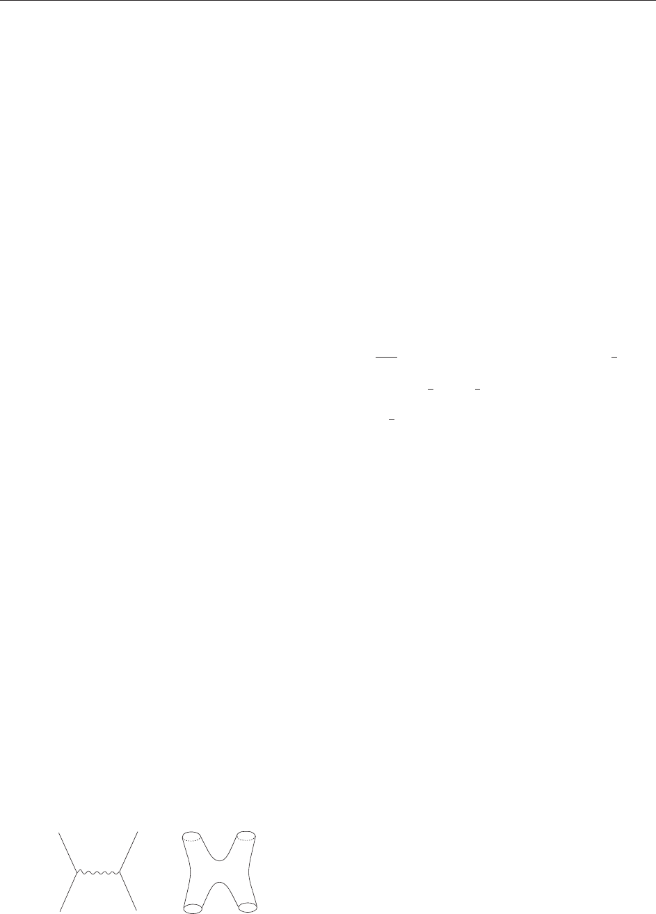
Strings interact by splitting or by joining at a point,

as is illustrated in Figure 1. This is a local

interaction that respects the causality of the theory.

To compute scattering amplitudes, one sums over all

world sheets with a given set of asymptotic states,

and weighs each local interaction with a factor of

the string coupling constant . The expansion in

powers of  is analogous to the Feynman-diagram

expansion of point-particle field theories. These

latter are usually defined by a Lagrangian, or more

exactly by a functional-integral measure, and they

make sense both for off-shell quantities as well as at

the nonperturbative level. In contrast, our current

formulation of superstring theory is in terms of a

perturbatively defined S-matrix. The advent of

dualities has offered glimpses of an underlying

nonperturbative structure called M-theory, but

defining it precisely is one of the major outstanding

problems in the subject. (One approach consists in

trying to define a second-quantized string field

theory; see String Field Theory).

Another important expansion of string theory,

very useful when it comes to extracting spacetime

properties, is in terms of the characteristic string

length l

ﬃﬃﬃﬃﬃ



. At energy scales El

 1, only a

handful of massless string states propagate, and their

interactions are governed by an effective low-energy

Lagrangian. In the type II theories, the massless

bosonic states (or rather their corresponding fields)

consist of the metric G



, a scalar field  called the

dilaton, and a collection of antisymmetric n-form

fields coming from both the NS–NS and the R–R

sectors. For type IIA, these latter are an NS–NS

2-form B

, an R–R 1-form C

, and an R–R 3-form

. The leading-order action for these fields reads:

IIA

2



ﬃﬃﬃﬃﬃﬃﬃﬃ

G

2

ðR þ4@



@



 



ﬃﬃﬃﬃﬃﬃﬃﬃ

G

C





½6

where F

=dC

, H

=dB

, and F

=dC

are field

strengths, the wedge denotes the exterior product of

forms, and jF

=(1=n!)F









. The dimen-

sionful coupling  can be expressed in terms of the

string-theory parameters, 2

=(2)





. A similar

expression can be written for the IIB theory, whose

R–R sector contains a 0-form, a 2-form, and a

4-form potential, the latter with self-dual field

strength.

The action [6], together with its fermionic part,

defines the maximally supersymmetric nonchiral

extension of Einstein’s gravity in ten dimensions

called type IIA supergravity (see Supergravity and

Salam and Sezgin (1989)). The dilaton and all

antisymmetric tensor fields belong to the super-

multiplet of the graviton – they provide together the

same number of (bosonic) states as a ten-dimensional

nonchiral gravitino. Supersymmetry fixes further-

more completely all two-derivative terms of the

action, so that the theory defined by [6] is (almost)

unique. (There exists in fact a massive extension of

IIA supergravity, which is the low-energy limit of

string theory with a nonvanishing R–R 10-form field

strength.) It is, therefore, not surprising that it should

emerge as the low-energy limit of the (nonchiral)

superstring theory. The latter provides, however, an

ultraviolet completion of an otherwise nonrenorma-

lizable theory, a completion which is, at least

perturbatively, finite and consistent.

Figure 1 A four-particle and a four-string interaction.

Superstring Theories 135

The finiteness of string perturbation theory has

been, strictly speaking, only established up to two

loops – for a recent review see D’Hoker and Phong

(2002). However, even though the technical pro-

blem is open and hard, the qualitative case for all-

order finiteness is convincing. It can be illustrated

with the torus diagram which makes a one-loop

contribution to string amplitudes. The thin torus of

Figure 2 could be traced either by a short, light

string propagating (virtually) for a long time, or by a

long, heavy string propagating for a short period of

time. In conventional field theory, these two virtual

trajectories would have made distinct contributions

to the amplitude, one in the infrared and the second

in the ultraviolet region. In string theory, on the

other hand, they are related by a modular transfor-

mation (that exchanges 

with 

) and must not,

therefore, be counted twice. A similar kind of

argument shows that all potential divergences of

string theory are infrared – they are therefore

kinematical (i.e., occur for special values of the

external momenta), or else they signal an instability

of the vacuum and should cancel if one expands

around a stable ground state.

The low-energy limit of the heterotic and type I

string theories is N = 1 supergravity plus super

Yang–Mills. In addition to the N = 1 graviton

multiplet, the massless spectrum now also includes

gauge bosons and their associated gauginos. The

two-derivative effective action in the heterotic case

reads:

het

2

ﬃﬃﬃﬃﬃﬃﬃﬃ

G

2



R þ 4@



@



 þ



trðF







gauge



þ fermions ½7

where !

gauge

= tr(AdA þ (2=3)A

) is the Chern–

Simons gauge 3-form. Again, supersymmetry fixes

completely the above action – the only freedom is in

the choice of the gauge group and of the Yang–Mills

coupling g

. Thus, up to redefinitions of the fields,

the type I theory has necessarily the same low-

energy limit.

The D = 10 supergravity plus super Yang–Mills

has a hexagon diagram that gives rise to gauge and

gravitational anomalies, similar to the triangle

anomaly in D = 4. It turns out that for the two

special groups E

 E

and SO(32), the structure of

these anomalies is such that they can be canceled by

a combination of local counter-terms. One of them

is of the form

^ X

(F, R), where X

is an 8-form

quartic in the curvature and/or Yang–Mills field

strength. The other is already present in the lower

line of expression [7], with the replacement

gauge

 !

Lorentz

, where the second Chern–

Simons form is built out of the spin connection.

Note that these modifications of the effective action

involve terms with more than two derivatives, and

are not required by supersymmetry at the classical

level. The discovery by Green and Schwarz that

string theory produces precisely these terms (from

integrating out the massive string modes) was called

the ‘‘first superstring revolution.’’

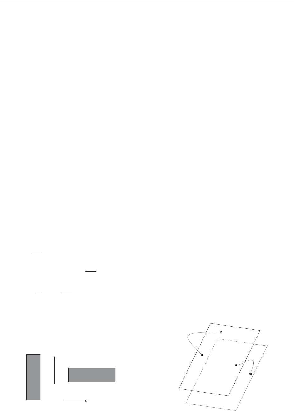
D-Branes

A large window into the nonperturbative structure

of string theory has been opened by the discovery of

D(irichlet)-branes, and of strong/weak-coupling

duality symmetries. A Dp brane is a solitonic

p-dimensional excitation, defined indirectly by the

property that open string endpoints can attach to its

world volume (see Figure 3). Stable Dp branes exist

in the type IIA and type IIB theories for p even,

respectively, odd, and in the type I theory for p = 1

and 5. They are charged under the R–R (p þ 1)-form

potential or, for p > 4, under its magnetic dual.

Strictly speaking, only for 0  p  6 do D-branes

resemble regular solitons the word stands for

‘‘solitary waves’’). The D7 branes are more like

Time

Space

Figure 2 The same torus diagram viewed in two different

channels.

Figure 3 D-branes and open strings.

136 Superstring Theories

cosmic strings, the D8 branes are domain walls,

while the D9 branes are spacetime filling. Indeed,

type I string theory can be thought as arising from

type IIB through the introduction of an orientifold

9-plane (required for tadpole cancelation) and of 32

D9 branes.

The low-energy dynamics of a Dp brane is

described by a supersymmetric abelian gauge theory,

reduced from ten down to p þ 1 dimensions. The

gauge field multiplet includes 9  p real scalars,

plus gauginos in the spinor representation of the

R-symmetry group SO(9  p). These are precisely

the massless states of an open string with endpoints

moving freely on a hyperplane. The real scalar fields

are Goldstone modes of the broken translation

invariance, that is, they are the transverse coordinate

fields

Y(

) of the D-brane. The bosonic part of the

low-energy effective action is the sum of a Dirac–

Born–Infeld (DBI) and a Chern–Simons (CS) like

term:

¼T

pþ1

 e



ﬃﬃﬃﬃﬃﬃﬃﬃﬃﬃﬃﬃﬃﬃﬃﬃﬃﬃﬃﬃﬃﬃﬃﬃﬃﬃﬃﬃﬃﬃﬃﬃﬃﬃﬃﬃ

detð

þF

 

^ e

½8

where F

þ 2

, hats denote pullbacks

on the brane of bulk tensor fields (e.g.,







), F

is the field strength of the

world-volume gauge field, and in the CS term

one is instructed to keep the (p þ 1)-form of the

expression under the integration sign. The constants

and 

are the tension and charge density of the

D-brane. As was the case for the effective super-

gravities, the above action receives curvature

corrections that are higher order in the 

expan-

sion. Note however that a class of higher-order

terms have been already resummed in expression

[8]. These involve arbitrary powers of F

, and are

closely related more precisely T-dual, see later) to

relativistic effects which can be important even in

the weak-acceleration limit. When refereing to the

D9 branes of the type I superstring, the action [8]

includes the GS terms required to cancel the gauge

anomaly.

The tension and charge density of a Dp brane can

be extracted from its coupling to the (closed-string)

graviton and R–R (p þ 1)-form, with the result:

¼ 





ð4



3p

½9

The equality of tension and charge follows from

unbroken supersymmetry, and is also known as a

Bogomol’nyi–Prasad–Sommerfeld (BPS) condition.

It implies that two or more identical D-branes

exert no net static force on each other, because

their R–R repulsion cancels exactly their gravita-

tional attraction. A nontrivial check of the result

[9] comes from the Dirac quantization condition

(generalized to extended objects by Nepomechie

and Teitelboim). Indeed, a Dp brane and a

D(6  p)-brane are dual excitations, like electric

and magnetic charges in four dimensions, so their

couplings must obey

2



6p

¼ 2k where k 2 Z ½10

This ensures that the Dirac singularity of the long-

range R–R fields of the branes does not lead to an

observable Bohm–Aharonov phase. The couplings

[9] obey this condition with k = 1, so that D-branes

carry the smallest allowed R–R charges in the

theory.

A simple but important observation is that open

strings living on a collection of n identical D-branes

have matrix-valued wave functions

, where

i, j = 1, ..., n label the possible endpoints of the

string. The low-energy dynamics of the branes is

thus described by a nonabelian gauge theory, with

group U(n) if the open strings are oriented, and

SO(n) or Sp(n) if they are not. We have already

encountered such Chan–Paton factors in our discus-

sion of the type I superstring. More generally, this

simple property of D-branes has led to many insights

on the geometric interpretation and engineering of

gauge theories, which are reviewed in the articles

Brane Construction of Gauge Theories and Gauge

Theories from Strings. It has also placed on a firmer

footing the idea of a brane world, according to

which the fields and interactions of the standard

model would be confined to a set of D-branes, while

gravitons are free to propagate in the bulk (for

reviews, see Brane Worlds and reference Lust

(2004)). It has, finally, inspired the gauge/string

theory or AdS/CFT correspondence (see Ads/CFT

Correspondence and Aharony et al. (2000))on

which we will comment later.

Dualities and M Theory

One other key role of D-branes has been to provide

evidence for the various nonperturbative duality

conjectures. Dual descriptions of the same physics

arise also in conventional field theory. A prime

example is the Montonen–Olive duality of four-

dimensional, N = 4 supersymmetric Yang–Mills,

which is the low-energy theory describing the

dynamics of a collection of D3 branes. The action

Superstring Theories 137