Francoise J.-P., Naber G.L., Tsun T.S. (editors) Encyclopedia of Mathematical Physics
Подождите немного. Документ загружается.

in the case with magnetic field. This can be made
rigorous (see Jerrard and Soner (2002) and Sandier
and Serfaty (to appear)), that is, one can expres s that
curl hiu; rui2
X
i
d
i
a
i
! 0as" ! 0 ½10
(or respectively curlhi , r
A
iþcurlA 2
P
i
d
i
a
i
! 0) in some weak functional norm, thus giving a
rigorous use of [8]. The quantity
ðuÞ¼curl hiu; rui½11
or
ð ; AÞ¼curl hi ; r
A
iþcurl A ¼ curl j þ h ½12
in the case with magnetic field, will thu s be called
the vorticity and be used to trace the vortices, in this
limit " ! 0. The relation
2
X
i
d
i
a
i
! 0as" ! 0 ½13
states that it is close to being a measure.
This is also called the Jacobian determinant if
written (with differential forms) Ju = dhiu,dui=
hidu,dui= 2(u
x
1
u
x
2
)dx
1
^ dx
2
, and unde r this
form it can be used in higher dimensions.
The Cost of Each Vortex
Here we investigate informally the cost of a vortex
of degree d. We know already that the characteristic
length scale of variation of u is ", and that (1
juj
2
)
2
is strongly penalized. Thus, we may expect
that juj is close to 1 at a distance " of the zeros.
Assuming that x
0
is a zero of u, and taking formally
juj= 1 for jx x
0
j", we may write u = e
i’
and
jruj= jr’j for jx x
0
j".
Then, we have
1
2
Z
Rjxx
0
j"
jruj
2
1
2
Z
R
"
Z
@Bðx
0
;rÞ
@’
@
2
!
dr
1
2
Z
R
"
Z
@Bðx
0
;rÞ
@’
@
!
2
1
2r
0
@
1
A
dr ½14
1
2
4
2
d
2
2
Z
R
"
dr
r
¼ d
2
log
R
"
½15
where we have used the Cauchy–Schwarz inequality
for [14], and the characterization of the degree [7].
We may also observe that this lower bound is sharp
if @’=@ is constant, that is, if the phase is d (and
the vortex radial). The cost associated to juj in the
energy imposes the length scale " and is generally of
order 1 (jrujC="), thus negligible compared to
the cost associated to the phase, which blows up as
log 1=" as " ! 0.
The above estimate is only valid as long as
B(x
0
, R) does not contain any other zero of u.If
vortices get close to each other or become numer-
ous, one needs refined techniques to estimate their
cost. This can be done through a ‘‘ball-construction
method’’ introduced independently by Jerrard and
Sandier.
Evaluating the Total Interaction Cost of Vortices
In a first approach, one studies configurations which
satisfy the upper bound E
"
(u) Cjlog "j. Then,
lower bounds of the type [15] show that the total
sum of the degrees (hence the total number of
vortices of nonzero degree) remains bounded as " ! 0.
Up to extraction, we may assume these zeros a
i
converge as " ! 0 to a finite set of points p
i
,witha
total degree still denoted d
i
. This can also be expressed
as (u
"
) ! 2
P
i
d
i
p
i
as " ! 0.
This is not the only case of interest, since
unbounded numbers of vortices do arise, especially
in the physical situation of the energy with magnetic
field, as we will see in the next section. However,
this hypothesis, which was made in the work of
Bethuel–Brezis–He´lein, makes the analysis easier
and already allows us to exhibit the main
phenomena.
Vortices in superconductors are generated by the
presence of the external magnetic field h
ex
. For the
energy without magnetic field, this has to be
replaced by some boundary condition which forces
some degree. Bethuel–Brezis–He´lein considered the
fixed Dirichlet boundary condition u
"
= g on @,
where g is a fixed unit-valued map on @, of degree
d >0. This forces u to have a total degree d in .
However, the Neumann boundary condition, for
instance, can also be considered (the minimizers of
E
"
are then simply con stants, they are trivial, but
one can still look for other critical points).
Let us return to lower bounds in order t o look
for the next order term in the energy (still with
formal arguments). Cutting out holes [
i
B(p
i
, )of
fixed size around the limiting vortices p
i
,wemay
assume that u = e
i’
in n[
i
B(p
i
, ) =
,with’ a
real-valued function, defined modulo 2. Minimiz-
ing the energy outside of the holes amounts to
solving
min
u:
!S
1
u¼g on @
degðu;@Bðp
i
;ÞÞ¼d
i
1
2
Z
jruj
2
358 Variational Techniques for Ginzburg–Landau Energies
This is a harmonic map proble m, whose solution is
given in terms of ’ by
’ ¼ 0in
@’
@
¼ ig;
@g
@
on @
Z
@Bðp
i
;Þ
@’
@
¼ 2d
i
and in terms of the harmonic conjugate which is
the function (up to a constant) such that
r’ = r
?
,
¼ 0in
@
@
¼ ig;
@g
@
on @
Z
@Bðp
i
;Þ
@
@
¼ 2d
i
½16
As ! 0, behaves like the solution of
0
¼ 2
X
i
d
i
p
i
in
@
0
@
¼ ig;
@g
@
on @
½17
Hence, we have
1
2
Z
jr’j
2
¼
1
2
Z
jrj
2
’
1
2
Z
jr
0
j
2
¼
X
i
d
2
i
log
1
þ W
d
ðp
1
; ...; p
n
Þ
þ oð1Þ as ! 0 ½18
where
W
d
ða
1
; ...; a
n
Þ¼
X
i6¼j
d
i
d
j
log jp
i
p
j
j
X
i
d
i
Rða
i
Þ
þ
1
2
Z
@
0
ig;
@g
@
½19
and R(x) =
0
(x)
P
i
d
i
log jx p
i
j. The function
W was introduced by Bethuel–Brezis–He´lein and
called the renormalized energy, since it consists in
the part of the energy that is left after subtracting
the ‘‘infinite part’’ in jlog "j from E
"
. It contains the
(logarithmic) interaction energy between the vor-
tices: we see that vortices with degrees of same sign
repel one another while vortices with degrees of
opposite signs attract one another. The d
2
i
log 1=
term corresponds to the self-interaction, or cost of
the vortex of core of size ; it is what replaces the
infinite term in the formal calculation.
Now [18] is a good estimate for the optimal
energy outside of the holes, while the energy in holes
of size can be bounded below by [15]. Given the
degree d
i
on the boundary @B(p
i
, ) of the small
hole, B(p
i
, ) contains one or several zeros of u of
degrees
k
with total degree
P
k
k
= d
i
. In view of
[15], since the cost of a vortex of degree d grows like
d
2
jlog "j, and since the infimum of
P
k
2
k
under the
constraint
P
k
k
= d
i
is
k
= sign(d
i
), the least costly
way to achieve this is to have jd
i
j vortices of degree
sign(d
i
). The smallest lower bound possible is thus
1
2
Z
Bðp
i
;Þ
jruj
2
þ
ð1 juj
2
Þ
2
2"
2
j d
i
jlog
"
þ C ½20
where the constant C can be described explicitly.
Adding up the results of [20] and [18], we find
E
"
ðuÞ
X
i
d
2
i
log
1
þ
X
i
jd
i
jlog
"
þ W
d
ðp
1
; ...; p
n
Þ
þ nC þ o
ð1Þþo
"
ð1Þ
X
i
jd
i
jlog
1
"
þ W
d
ðp
1
; ...; p
n
Þ
þ nC þ o
"
ð1Þ½21
with equality only if u has jd
i
j zeros of degree
sign(d
i
) in each B(p
i
, ).
This provides a lower bound of the energy in
terms of the vortices. Moreover, this bound is sharp:
one can construct test confi gurations which have the
given limiting vortices (p
i
, d
i
), and an energy equal
to the right-hand side of [21].
One can thus deduce the behavior of global
minimizers of the energy. Give n the total degree
d = deg(g)>0on@ ,weneed
P
i
d
i
= d,andthe
lowest value achievable under this constraint in
the right-hand side of [21] is to have d
i
= 1for
every i, and thus to have exactly d vortices of
degree 1. Moreover, the limiting points p
i
’s
should minimize W. We thus are led to the first
main result.
Theorem 1 (Bethuel–Brezis–He´lein). Minimizers of
E
"
under the boundary condition u = g,deg(g) = d > 0,
have d zeros of degree 1, which converge as " ! 0
to a minimizer of W.
This result can be rephrased as a result of
-convergence of E
"
djlog "j. It reduces the
minimization of E
"
to one of W, which is a finite-
dimensional problem (interaction of point charges).
Variational Techniques for Ginzburg–Landau Energies 359

Thus, we see again the interest of studying this
asymptotic limit " ! 0 because the vortices become
pointlike and the problem reduces to a finite-
dimensional one, or one of minimizing the vortex
interaction.
Further Results
A nonvariational approach also allowe d Bethuel–
Brezis–He´lein to prove a further correspondence
between E
"
and W: they obtained that critical points
of E
"
, under the upper bound E
"
Cjlog "j, have
vortices which con verge to a critical point of W.
Other important resul ts are the study of the blow-up
profiles or solutions in the whole plane, by Brezis–
Merle–Rivie` re and Mironescu.
In two dimensions, the variational approach is
also used to solve inverse problems (construct
solutions) and study variants of the energy with
pinning (or weighted) terms.
The variational approach is also fruitful in higher
dimensions. In dimension 3, for example, vortices are
not points but vortex lines, and the Jacobian
Ju = d(iu,du) can be seen as a current carried by the
vortex line, with kJuktotal mass of the current equal to
times the length of the line, and it was established by
Jerrard and Soner that Ju
"
is compact in some weak
sense, and converges, up to extraction, to some times
integer-multiplicity rectifiable current J,with
lim inf
"!0
E
"
ðu
"
Þ
jlog "j
kJ k
In fact, a compl ete -convergence result of
E
"
=jlog "j can be proved, see the work of Alberti–
Baldo–Orlandi, and thus minimizing E
"
reduces at
the limit to minimizing the length of the line, leading
to straight lines, or in higher dimensions, to
codimension-2 minimal currents. This is a nontrivial
problem, contrarily to dimension 2, where the -
limit of E
"
=jlog "j is trivial, which required to go to
the lower-order term to find the nontrivial renorma-
lized energy limit W.
The Functional with Magnetic Field
The aim here is to achieve the same objective:
express or bound from below the energy by terms
which depend only on the vortices and their degrees.
The method consists in transposing the type of
analysis above taking into account the magnetic
field contribution to see how the external field
triggers the sudden appearance of vortices, and for
what values they appear (thus retrieving the critical
fields, etc.). One of the main difficulties consists in the
fact that the number of vortices becomes divergent,
which requires more delicate estimates. Also, it is then
no longer possible to study the convergence of the
individual zeros of , so one studies instead the limit of
rescalings of the vorticity measures ( , A).
Splitting of the Energy and Main Results
Let us recall that in the case with magnetic field, the
vorticity is given by [12]. In addition, we may
assume that the second set of equations in [5]
r
?
h ¼ j in ; h ¼ h
ex
on @ ½22
is satisfied (if not, keeping fixed and choosing A
which satisfies this equation always decreases the
energy). Taking the curl of this equation, we find
exactly
h þ h ¼ ð ; AÞ in
h ¼ h
ex
on @
½23
Thus, the vorti city and the induced magnetic field
are in one-to-one correspondence with each other.
Combining it to the relation [13], we are led to the
approximate relation
h þ h ’ 2
X
i
d
i
a
i
in
h ¼ h
ex
on @
½24
where again the a
i
’s are the vortex centers and d
i
’s
their degrees, well known in physics as the
‘‘London equation.’’ It shows how the magnetic
field is induced by the vortices which act like
‘‘charges,’’ and how the magnetic field ‘‘penetrates
the sample’’ around the positive vortex locations.
Of course this equation is only an approximation,
because the singularities at the a
i
’s, where h would
become infinite, are really smoothed out in ( , A);
however, the approximation is good far f rom
the vortex cores, just as [17] is an approximation
for [16].
It is then natural to introduce the field corre-
sponding to the vortex-free situation, which is h
ex
h
0
where h
0
solves
h
0
þ h
0
¼ 0in
h
0
¼ 1on@
½25
h
0
is thus a fixed smooth function, depending only
on , and when there are no vortices, we expect h to
be approximately h
ex
h
0
. Moreover, h
0
:= h h
ex
h
0
then solves
h
0
þ h
0
¼ ð ; AÞ’2
X
i
d
i
a
i
in
h
0
¼ 0on@
½26
360 Variational Techniques for Ginzburg–Landau Energies
Defining the Green kernel G(. , y)by
G þ G ¼
y
in
G ¼ 0on@
½27
and S by S(x, y) = 2G(x, y) þ log jx yj,forx far
enough from the a
i
’s, we may approximate h
0
by
h
0
ðxÞ¼2
X
i
Gðx; a
i
Þ½28
Using the second Ginzburg–Landau equation [22]
and the fact that j j1, we have jr
A
jjjj= jrhj,
thus G
"
( , A) (1=2)
R
jrhj
2
þjh h
ex
j
2
. Plugging
in the decomposition h = h
ex
h
0
þ h
0
and using an
integration by parts and [26], one finds
G
"
ð ; AÞ¼
1
2
h
2
ex
Z
jrh
0
j
2
þjh
0
1j
2
þ h
ex
Z
rh
0
rh
0
þðh
0
1Þh
0
þ
1
2
Z
jrh
0
j
2
þjh
0
j
2
¼ h
2
ex
J
0
þ h
ex
Z
ðh
0
1Þð ; AÞ
þ
1
2
Z
jrh
0
j
2
þjh
0
j
2
½29
where J
0
is the constant (1=2)
R
jrh
0
j
2
þjh
0
1j
2
.
The right-hand side of eqn [29] can be expressed
in terms of the vortices. First, using [26],we
have
R
(h
0
1)( , A) ’2
P
i
d
i
(h
0
1)(a
i
). Second,
the expression
R
jrh
0
j
2
þjh
0
j
2
can be treated exactly
like E
"
(u) in the previous section, using lower bounds for
the cost of vortices provided by the Jerrard–Sandier
method, we are led to the (approximate) relation
1
2
Z
jrh
0
j
2
þjh
0
j
2
X
i
jd
i
jlog
1
"
X
i6¼j
d
i
d
j
log ja
i
a
j
j
þ
X
i;j
d
i
d
j
Sða
i
; a
j
Þ½30
Combining this to [29] we find the decomposition
G
"
ð ; AÞh
2
ex
J
0
þ
X
i
jd
i
jjlog "j
þ 2h
ex
X
i
d
i
ðh
0
1Þða
i
Þ
X
i6¼j
d
i
d
j
log ja
i
a
j
j
þ
X
i;j
d
i
d
j
Sða
i
; a
j
Þ½31
On the other hand, this inequality is sharp: as
before, given vortices a
i
, one can construct a
configuration ( , A) for which this is an equality,
at leading order.
In that relation, h
2
ex
J
0
is a fixed energy, the energy
of the vortex-free configuration. To it are added the
intrinsic cost of each vortex jd
i
jjlog "j , the interac-
tion cost between vortices, and the interaction
between the vortices and the external field
2h
ex
P
i
d
i
(h
0
1)(a
i
).
It is then simple, by minimizing the right-hand
side with respect to the vortices for a given h
ex
, and
observing that h
0
1 0, to deduce a few basic
facts about vortices: vortices of positive degree (and
of degree þ1) are preferred, each vo rtex costs
jlog "j, an d allows to gain at best an energy
2h
ex
max jh
0
1j when placed at the minimum of
h
0
1. Therefore, vortices become favorable when
their cost becomes smaller than the gain, that is,
when h
ex
becomes larger than the ‘‘first critical field’’
H
c
1
jlog "j
2jminðh
0
1Þj
½32
We have the first main result.
Theorem 2 (Sandier–Serfaty). When " is small
enough and h
ex
H
c
1
, then minimizers of G
"
have
no vortices.
On the other hand, if h
ex
H
c
1
, the vortices
cannot all be located at the same minimum point of
h
0
1, because their repulsion
P
i6¼j
log ja
i
a
j
j
would be infinite. There is thus a trade-off between
their repulsion and the cost for being far from the
minimum of h
0
1. Only if n, the number of
vortices, is small compared to h
ex
do the vortices
tend to concentrate near the minimum of h
0
1. If
so, then, assuming for simplicity that the minimum
of h
0
1 is achieved at a unique point p, and
denoting by Q the Hessian of h
0
1atp,inthe
relation above (h
0
1)(a
i
) can be approximated by
min (h
0
1) þ (1=2)Q(a
i
p) and thus G
"
( , A)by
G
"
ð ;AÞh
2
ex
J
0
þnjlog "jþ2nh
ex
minðh
0
1Þ
þh
ex
X
i
Qða
i
pÞ
X
i6¼j
d
i
d
j
logja
i
a
j
jþn
2
Sðp;pÞ½33
From this relation, optimizing on ‘, the character-
istic distance to p and characteristic distance
between the vortices, we find that ‘ =
ffiffiffiffiffiffiffiffiffiffiffiffi
n=h
ex
p
is
optimal.
Moreover, optimizing with respect to n, we find
that n should remain bounde d (as " ! 0) when
h
ex
H
c
1
þ O( log jlog "j). In that regime, rescaling
by setting x
i
= ((a
i
p)=‘), we have the following
result:
Variational Techniques for Ginzburg–Landau Energies 361
Theorem 3 (Sandier–Serfaty). There exist fields
H
n
H
c
1
þ C(n 1) log jlog "j such that when
H
n
h
ex
< H
nþ1
, minimizers of G
"
have n vortices
of degree 1, and the rescaled vortices x
i
’s tend to
minimize:
w
n
ðx
1
; ...; x
n
Þ¼
X
i6¼j
log jx
i
x
j
j
þ n
X
n
i¼1
Qðx
i
Þ½34
If h
ex
H
c
1
log jlog "j, then the optimal number
of vortices n becomes unbounded as " ! 0. The
analysis above still holds, but in order to get a
convergence of the vortices, one needs to rescale the
vorticity measure by n. There is an intermediate
regime, for log jlog "jh
ex
H
c
1
jlog "j for
which n should be 1 but still n h
ex
,so‘ 1:
vortices are numerous, but still concentrate around p.
Rescaling by the scale ‘ as above, we prove that the
density of vortices (after dividing it by n)convergesto
a probability measure, minimizer of the energy
IðÞ¼
Z
R
2
R
2
log jx yjdðxÞdðyÞ
þ
Z
R
2
QðxÞdðxÞ½35
This is an averaged/continuous form of [34].
If h
ex
H
c
1
is of order jlog "j, then the optimal
number n becomes of order h
ex
and the vortices no
longer concentrate around a single point.
The simplest approach is then to simply consider
the vorticity measure ( , A) and to rescale it by the
order n, hence by h
ex
. Then (1=h
ex
)( , A) con-
verges, after extraction, to some measure
.A
continuous version of [31] can thus be written, using
[12],as
G
"
ð ;AÞ
1
2
h
ex
jlog "j
Z
j
jþ
1
2
h
2
ex
Z
jrh
j
2
þjh
j
2
½36
where h
solves
h
þ h
¼
in
h
¼ 1on@
Again, this inequality can be proved to be sharp (by
a construction) and allows to show that minimizers
of G
"
have a vorticity ( , A) such that ( , A)=h
ex
converges to a minimizer of
Gð
Þ¼
1
2
lim
"!0
jlog "j
h
ex
Z
j
jþ
1
2
Z
jrh
j
2
þjh
j
2
In fact the stronger result holds, in that sense:
Theorem 4 (Sandier–S erfaty). G
"
=h
2
ex
-converges
to G.
The limit pr oblem of minimizing G turns out to
have a simple solution in terms of an obstacle
problem: the optimal
is a uniform density of
vortices on a subdomain of determined through a
free boundary problem (and depending on h
ex
),
which is nonzero.
In all these regimes, we have thus been able to
identify the optimal number and repartition of
vortices through a -convergence-type approach,
that is, by reducing the minimization of the energy
to the minimization of a limiting problem: w
n
or I or G,
according to the regime.
Further Results
Concerning vortices, in the same spirit as what was
done for E
"
, we can obtain necessary conditions
characterizing limiting vorticities obtained from
sequences of (nonminimizing) critical points of
the energy G
"
. They consist in passing to the limit
in the conservative form of the Ginzburg–Landau
equations [5].
Most of the results concerning the phase transi-
tions at the next critical fields H
c
2
and H
c
3
are also
obtained by nonvariational methods, and often by
linear analysis.
The study of the Ginzburg–Landau energy in non-
simply-connected domains is also very interesting
because it leads to nontrivial topological effects, since
in such domains there exist unit-valued maps with
nonzero degree (corresponding to permanent currents).
See also: Abelian Higgs Vortices; Aharonov–Bohm Effect;
Bose–Einstein Condensates; Gamma-Convergence and
Homogenization; Gauge Theory: Mathematical
Applications; Ginzburg–Landau Equation; High T
c
Superconductor Theory; Image Processing:
Mathematics; Superfluids; Topological Defects and Their
Homotopy Classification; Variational Techniques for
Microstructures.
Further Reading
Bethuel F, Brezis H, and He´lein F (1994) Ginzburg–Landau
Vortices. Boston: Birkha¨ user.
DeGennes PG (1966) Superconductivity of Metal and Alloys.
New York: Benjamin.
Jerrard RL and Soner HM (2002) The Jacobian and the
Ginzburg–Landau energy. Calculus of Variations and Partial
Differential Equations 14(2): 151–191.
Sandier E and Serfaty S Vortices in the Magnetic Ginzburg–
Landau Model. Birkha¨ user (monograph to appear).
Tinkham M (1996) Introduction to Superconductivity, 2nd edn.
McGraw-Hill.
362 Variational Techniques for Ginzburg–Landau Energies
Variational Techniques for Microstructures
G Dolzmann, University of Maryland, College Park,
MD, USA
ª 2006 Elsevier Ltd. All rights reserved.
Austenite–Martensite Transformations
and the Shape Memory Effect
Microstructures in materials that typically form in
response to phase transformations in the solid state,
and their impact on the elastic properties of these
materials have been known for centuries. The
discovery of the complex phase diagram of iron
revolutionized the production of steels at the end of
the nineteenth century. Starting in the 1980s, the
mathematical description of microstructures in the
framework of nonlinear elasticity has led to deep
analytical questions and surprising developments in
the calculus of variations and in nonlinear partial
differential equations.
The mathematical approach outlined here is based
on the following fundamental assumptions:
1. The observed configurations correspond to mini-
mizers of or elements of minimizing sequences
for an energy functional.
2. The qualitative properties of low energy states
are determined from the set of minima of the free
energy density.
Under these assumptions one aims at explaining
experimental observations and to predict material
properties based on minimizing an energy functional
of the form
IðuÞ¼
Z
WðDuÞdx
Here is an ideal, unstressed reference configura-
tion in R
n
, u : !R
m
is an elastic deformation, and
W : M
mn
!R is the stored energy density. In the
case of physical interest, m = n = 2orm = n = 3. For
applications in elasticity we assume that m = n, but
this assumption is not needed in the general theory.
The energy density W and its structure depend
critically on the temperature. However, since we are
interested in the analysis of the material at a given
temperature, we do not include this dependence
explicitly.
The key ingredient of this model is the stored
energy density W which has to reflect the properties
of the specific material one wants to model.
Frequently these are alloys, in particular shape
memory alloys that undergo an austenite–martensite
transformation. For most materials a closed analytic
expression for W is not available. In the spirit of the
fundamental assumption (2) one therefore focuses
on the structure of the set of minima of W which is
determined from general invariance and symmetry
principles. We may assume that W 0 and that
K = {X: W(X) = 0} 6¼;. The principle of material
frame indifference then asserts that
WðRFÞ¼WðFÞ for all R 2SOðnÞ
Here SO(n) is the group of proper rotations, that is,
the set of all matrices R 2M
nn
with R
T
R = Id and
det R = 1.
The symmetry of the austenitic (high-temperature)
phase implies that the energy density in the
martensitic (low-temperature) phase is invariant
under all changes of basis that leave the underlying
lattice in the austenitic phase invariant. Therefore,
WðR
T
FRÞ¼WðFÞ for all R 2P
a
where P
a
is the point group of the austenite. In the
case of a cubic to tetragonal phase transformation,
this leads to K = SO(3) in the austenitic phase and to
K ¼ SOð3ÞU
1
[ SOð3ÞU
2
[ SOð3ÞU
3
½1
with
U
i
¼
2
e
i
e
i
þ
1
I e
i
e
i
ðÞ½2
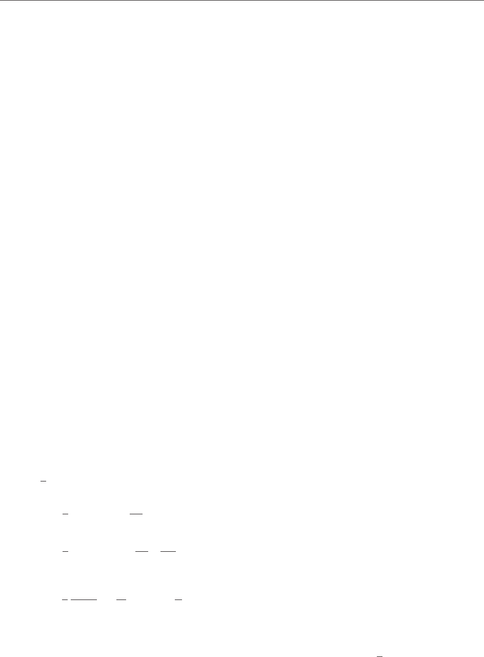
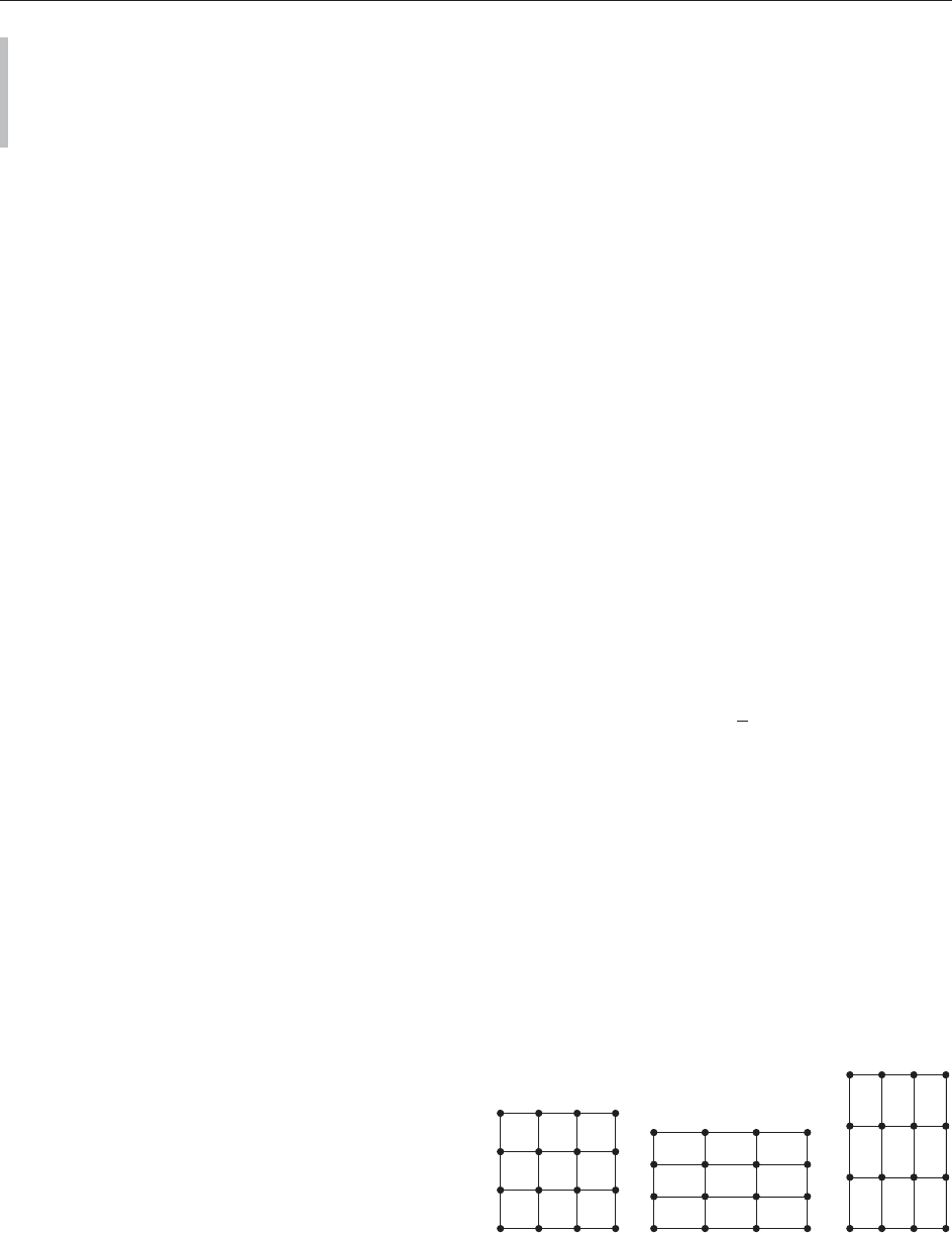
in the martensitic phase (see Figure 1). A set of the
form SO(n)U
i
is often referred to as an energy well.
The origin of the shape memory effect is the
availability of a rich class of geometric patterns in
which the martensitic phases can be arranged, thus
leading to a great flexibility of the material to
accommodate macroscopic deformations. Upon heat-
ing of the material above the transformation tem-
perature, the martensitic phases lose their stability
and the material returns to its unique shape in the
(a) (b) (c)
Figure 1 Two-dimensional cartoon of a cubic to tetragonal
phase transformation in a single crystal: (a) a cubic lattice, (b)
and (c) tetragonal variants which are stretched in directions e
1
and e
2
, respectively. (Sketch not to scale.)
Variational Techniques for Microstructures 363
austenitic phase. The two solutions of Hadamard’s
compatibility condition
QU
2
U
1
¼ a b; Q 2 SOð3Þ
are given by
Q
1
¼
1
4
þ 1
2
2
4
10
1
4
2
2
0
00
4
þ 1
0
@
1
A
½3
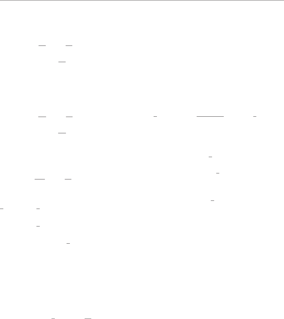
and Q
2
= Q
T
1
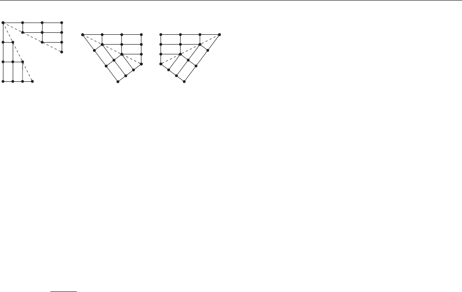
(see Figure 2). The normals (in the
reference configuration) are given by (1, 1, 0)=
ffiffiffi
2
p
.
It is one of the successes of the theory that it
provides an analytical derivation of the normals to
the twinning planes.
The Direct Method in the Calculus
of Variations
The mathematical interest in the variational prob-
lems described in the previous section lies in the fact
that existence of minimizers cannot in general be
obtained by a straightforward application of the
direct methods in the calculus of variations. This
approach is based on the idea to (1) choose a
minimizing sequence for the functional I, (2) show
that this sequence is bounded and precompact,
and (3) prove that the functional is lower semicon-
tinuous with respect to the notion of convergence,
IðuÞlim inf
j!1
Iðu
j
Þ if u
j
! u
The typical choice is to seek u
j
in a suitable Sobolev
space W
1, p
(; R
m
) with 1 < p 1which is related
to growth and coercivity conditions for the energy
density W,
c
1
jFj
p
c
2
WðFÞc
3
jF j
p
þ 1
for all F 2M
mn
½4
This leads to weak compactness in W
1, p
(; R
m
)
(weak- compactness in W
1, 1
(; R
m
)) and to the
requirement of sequential weak lower semicontinu-
ity of the functional,
IðuÞlim inf
j!1
Iðu
j
Þ if u
j
* u in W
1;p
ð; R
m
Þ
(sequential weak- lower semicontinuity for p = 1).
Morrey’s fundamental work establishes a link
between convexity conditions for the energy density
and lower semicontinuity of the variational integral:
under suitable growth and coercivity conditions,
sequential weak- lower semicontinuity is equivalent
to quasiconvexity of the integrand.
Definition 1 A function W : M
mn
!R is said to be
quasiconvex at F if
Z
WðFÞdx
Z
WFþ DðÞdx
for all 2W
1;1
0
ð; R
m
Þ
and for all open and bounded domains R
n
with
L
n
(@) = 0. It is said to be quasiconvex if it is
quasiconvex at all F.
In the language of nonlinear elasticity, W is
quasiconvex if affine functions are minimizers of
the energy functional subject to their own boundary
conditions. The direct method implies the following
classical existence theorem.
Theorem 1 Suppose that W : M
mn
!R is quasi-
convex and satisf ies the growth and coercivity
condition [4]. Let u
0
2W
1, p
(; R
m
). Then the varia-
tional problem: minimize I(u) in
A¼ u 2W
1;p
ð; R
m
Þ: u u
0
2W
1;p
0
ð; R
m
Þ
no
has a minimizer.
The remarkable fact is that the structure of the
zero set of a typical energy W modeling a phase-
transforming material in its low-temperature phase
prevents W from being quasiconvex. In order to see
this, let Q R
3
be a cube with two of its sides
perpendicular to b = (1, 1, 0)=
ffiffi
(
p
2) and let h be the
1-periodic function with h
0
= 0 on (0, )andh
0
= 1on
(, 1) with 2(0, 1). Define v
j
(x) = U
1
x þ ah( jx b)=j
and
u
j
ðxÞ¼min v
j
ðxÞ; distðx;@QÞ
¼ min U
1
x þ ahðjx bÞ=j; distðx;@QÞ
fg
where dist(x, @Q) = inf {kx yk
1
, y 2 @Q }. Then
u
j
!u, u(x) = Cx strongly in L
1
(Q; R
3
)andweakly-
in W
1, 1
(Q; R
3
)withC = U
1
þ (1 )Q
1
U
2
=2K
where K is the zero set of W, see the previous section.
(a) (b) (c)
Figure 2 Formation of phase boundaries in a single crystal.
(a) The upper right half of the lattice deforms into phase I with
the constant deformation gradient U
1
, the lower left half of the
lattice deforms into phase II with constant deformation gradient
U
2
: (b) An additional rotation is needed to accomplish a
continuous deformation, see formula [3]. (c) A different config-
uration with a different orientation of the interface. (Sketch not
to scale.)
364 Variational Techniques for Microstructures
Moreover, Du
j
2{U
1
, Q
1
U
2
} except in a small transi-
tion layer of volume O(1=j)closeto@Q and
IðuÞ¼
Z
WðCÞdx > lim inf
j!1
Iðu
j
Þ¼0
This inequality shows that the functional is not
weakly- lower semicontinuous and therefore W
fails to be quasiconvex. The oscillations of u
j
on a
scale 1=j are part of the mathematical model for the
microstructures frequently observed in shape mem-
ory alloys. More generally, whenever u is a Sobolev
function on a domain such that Du takes only two
values, say Du 2{A, B}, on open sets which are not
empty and whose union is (up to a set of measure
zero), then the tangential continuity of the deriva-
tives implies that the difference A B is a matrix of
rank 1, A B = a b, and that the interfaces
between the regions with Du = A and Du = B are
hyperplanes with normal parallel to b. This state-
ment is usually referred to as ‘‘Hadamard’s compat-
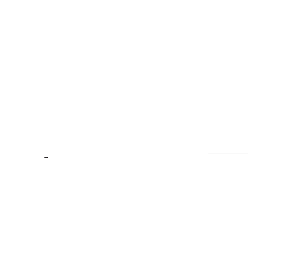
ibility condition.’’ Moreover, the pattern in Figure 3
is known as a ‘‘simple laminate’’ and the matrices A
and B are said to be rank-1 connected.
Relaxation
The discussion in the previous section shows that the
variational problems related to models in materials
science typically fail to be weakly lower semicon-
tinuous. One approach which allows us to recover
the macroscopic energy of the system and the macro-
scopic stress–strain relation is to pass to the relaxed
variational problem which involves the quasiconvex
envelope of the energy density W.
Definition 2 Let W : M
mn
!R be given. The
function
W
qc
¼ sup f : f W; f quasiconvex
fg
is called the quasiconvex envelope of W. Equivalently,
W
qc
ðFÞ¼ inf
2W
1;1
0
ð;R
m
Þ
1
jj
Z
WðF þ DÞdx
This formula implies that W
qc
is the macroscopic
energy of the system in the sense that it characterizes
the smallest energy per unit volume that is required
to subject a volume element to a deformation with
affine boundary conditions. Here the system is
allowed to minimize its energy with microstructures
at any scale, a mechanism which was already
explored in the previous section. The arguments in
this section prove that W
qc
(C) = 0 and this shows
that the zero set of W
qc
can be strictly larger than
the zero set of K, see Definition 4. The relaxed
functional is given by
I
qc
ðuÞ¼
Z
W
qc
ðDuÞdx
Since W
qc
satisfies the growth and coercivity
conditions [4] if they are satisfied by W,the
functional I
qc
attains its minimum subject to given
boundary conditions. The functional I
qc
is the
weakly lower semicontinuous envelope of I in the
sense that minimizing sequences for I contain
subsequences that converge to minimizers of I
qc
and for all u there exists a sequence u
j
which
converges in W
1, p
(; R
m
)tou such that the
energies converge, I(u
j
) !I(u). However, a lot of
information in particular about oscillation patterns
might be lost in the passage from I to I
qc
since the
knowledge of a minimizer u for I
qc
does not
provide any immediate information about the
behavior of any minimizing sequence for I that
converges to u. Moreover, the minimization pro-
blem required in the definition of the relaxed
energy has been solved explicitly only for very
special energy densities.
In this context, one often relies on two related
notions of convexity, one sufficient and the other
necessary for quasiconvexity. For F 2M
mn
let
M(F) 2 R
d(m, n)
be the vector of all minors (sub-
determinants) of F. In the special case m = n = 2
we have M(F) = (F, det F) 2R
5
and for m = n = 3
we find M(F ) = (F, cof F, det F) 2 R
19
where cof
F is the 3 3 matrix of all 2 2 subdeterminants
of F.
Definition 3 Let W : M
mn
!R be given. The
function W is said to be polyconvex if there exists
a convex function g : R
d(m, n)
!R such that
W(F) = g (M(F)). The function W isrank-1convexif
it is convex along all rank-1 lines in M
mn
,thatis,the
function t 7!W(F þ tR)isconvexforallF 2 M
mn
and all R 2 M
mn
with rank(R) = 1.
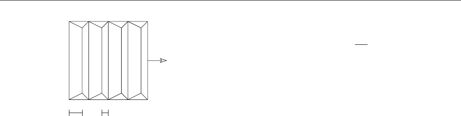
λ /j
BA
B
A
B
A
B
A
b
(1–λ)/j
Du
j
=
Figure 3 Construction of a minimizing sequence u
j
with Du
j
!
fA, Bg in measure and affine boundary conditions u(x) = A þ
(1 )B Hadamard’s compatibility condition requires that A
B = a b is a rank-1 matrix and that the planar interfaces are
perpendicular to b.
Variational Techniques for Microstructures 365
All notions of convexity reduce to classical
convexity if m = 1orn = 1. In the vector-valued
case m, n > 1 the following implications are true:
f convex ) f polyconvex ) f quasiconvex
) f rank-1 convex
The reverse statements for the first two implications
are not true. Rank-1 convexity does not imply
quasiconvexity for m 3 and it is a fundamental
open problem with deep connections to harmonic
analysis to decide whether rank-1 convexity and
quasiconvexity are equivalent for m = n = 2.
The polyconvex and the rank-1 convex envelope
of an energy density W are defined analogously to
Definition 2. In view of the implications between the
different notions of convexity, one has W
pc
W
qc
W
rc
and essentially all explicitly known
relaxation formulas are based on the approach to
construct a candidate W
for W
rc
and to verify that
W
is polyconvex. Then the inequalities become
equalities and one obtains a characterization for the
relaxed energy. This approach does not work for
extended-valued functions which are used in models
for incompressible materials since quasiconvexity
does not imply rank-1 convexity in this case.
However, for a model system of particular interest,
nematic elastomers, a complete characterization of
the relaxed energy, the macroscopic stress–strain
relation, and the macroscopic phase diagram have
been obtained.
Classical and Generalized Minimizers
The discussion of observed configurations as ele-
ments of minimizing sequences {u
j
} in the section
‘‘The direct method in the calculus of variations’’
leaves the question of the existence of minimizers
open. The answer cannot be obtained via the direct
methods since minimizing sequences do not need to
converge strongly to minimizers. One approach to
obtain the existence of solutions u with I(u) = 0isto
solve the differential relation Du 2K, u(x) = Fx on
@ by constructing special minimizing sequences
that converge strongly so that one can pass to
the limit in the energy integral. This idea has led
to surprising solutions u with affine boundary
conditions for the two-well problem where K =
SO(2)diag(,1=) [ SO(2)diag(1=, ). However, the
structure of the solutions is intrinsically complicated
in the sense that the phase boundary has infinite
length unless the boundary conditions are given by
u(x) = Fx with F 2K.
More generally, the right tool to pass to the limit in
nonlinear functions of z
j
= Du
j
like the energy is the
‘‘Young measure’’ generated by a subsequence. It is
given by a family of probability measures
x
that
provide statistical information about the distribution of
the values of z
j
close to a given point x. The existence
and the fundamental properties of Young measures are
described in the following theorem. For simplicity we
assume that the sequence z
j
is uniformly bounded.
Theorem 2 (Fundamental theorem on Young
measures). Let E R
n
be measurable, L
n
(E) < 1,
and let z
j
: E !R
d
be a measurable and bounded
sequence. Then there exists a subsequence z
k
and a
weakly- measurable map : E !M(R
d
) such that
the following assertions are true:
(i) The measures
x
are non-negative probability
measures.
(ii) If there exists a compact set K such that u
k
!K
in measure, then supp
x
K for a.e. x 2E.
(iii) If f 2C(R
d
) and if f(z
k
) is relatively weakly
compact in L
1
(E), then f (z
k
) * finL
1
(E)
where
f (x) = h
x
, f i.
Here h
x
, f i denotes the integration of the func-
tion f with respect to the measure
x
. For example,
the Young measure generated by the sequence Du
j
constructed in the section ‘‘The direct method in the
calculus of variations’’ generates the Young measure
x
= (1=2)
A
þ (1=2)
B
(see Figure 3) and
Iðu
j
Þ¼
Z
WðDu
j
Þdx
!
Z
Z
M
mn
WðYÞd
x
ðYÞdx ¼ 0
A Young measure generated by a sequence of
gradients is called a gradient Young measure
(GYM). It is said to be homogeneous if
x
= is
independent of x. We restrict our attention in the
following to homogeneous GYMs generated by
sequences that are bounded in L
1
. The importance
of quasiconvexity is also reflected in the following
characterization of homogeneous GYMs.
Theorem 3 A non-negative probability measure
is a GYM if and only if there exists a compact set
K M
mn
with supp K and Jensen’s inequality
h, f if (h,idi) holds for all quasiconvex functions
f : M
mn
!R.
This motivates to characterize the generalized
limits of minimizing sequences as
M
qc
ðKÞ¼ 2MðKÞ: f ðh; idiÞ h; f i
f
for all f : M
mn
! R quasiconvexg
where M(K) is the set of all probability measures
supported on K.If is generated by a sequence of
366 Variational Techniques for Microstructures
functions with affine boundary conditions
u
j
(x) = Fx, then h,idi= F. The set of all affine
deformations of the material that can be recovered
by heating (shape memory effect) is therefore given
as the set of all centers of mass of homogeneous
GYMs supported on K, the so-called ‘‘quasiconvex
hull’’ K
qc
of K.
Definition 4 Suppose that K M
mn
is compact.
We define the quasiconvex hull of K by
K
qc
¼ F ¼h; idi: 2M
qc
ðKÞ
fg
There are several equivalent definitions of K
qc
.
The foregoing definition corresponds to the defini-
tion of the convex hull of a set as the set of all
centers of mass of probability measures supported
on K (which satisfy Jensen’s inequality for all
convex f ). The set K
qc
can also be defined as the
set of all points that cannot be separated by
quasiconvex functions from K or as the zero set of
the quasiconvex envelope of the distance function to
K. The ‘‘polyconvex hull’’ K
pc
and the ‘‘rank-1
convex hull’’ K
rc
are defined analogously by replac-
ing quasiconvexity with polyconvexity and rank-1
convexity in the foregoing definitions. It follows that
K
rc
K
qc
K
pc
and all of these inclusions can be
strict.
A particularly useful set of conditions are the
minors conditions
h; Mi¼M h; idiðÞ
for all minors M which follow from the weak
continuity of the minors. For example, if
K = {A, B} M
22
, then any probability measure
supported on K is given by =
A
þ (1 )
B
. The
minors condition with M = det implies that
det A þð1 ÞBðÞ¼deth;idi¼h; deti
¼ det A þð1 Þdet B
This identity is equivalent to
ð1 ÞdetðA BÞ¼0
and therefore the quasiconvex hull is equal to K if
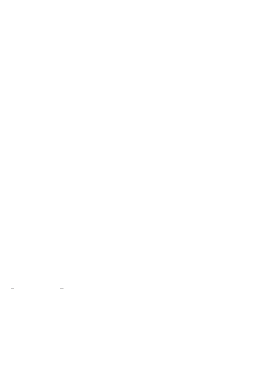
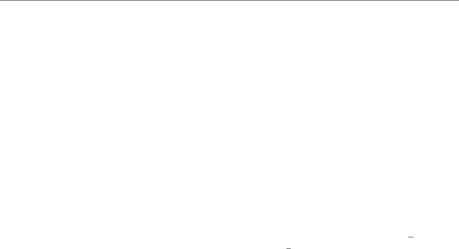
and only if det (A B) 6¼ 0. A very instructive
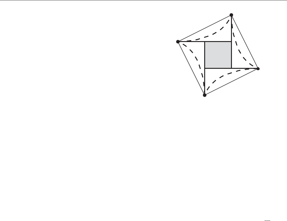
example is the set K = {(1, 3), (1, 3), (3, 1),
(3, 1)} viewed as a subset of the space of all
diagonal matrices in M
22
. It is frequently referred
to as a T
4
configuration. The rank-1 convex hull is
equal to the quasiconvex hull and given by the four
points, the line segments, and the square in the
center, the polyconvex hull is bounded by four
hyperbolic arcs, and the convex hull is the square
with the points as corners, see Figure 4.Itis
remarkable that the rank-1 convex hull is strictly
larger than the set K itself despite the fact that the
set K does not contain any rank-1 connections.
There are only a few examples in which explicit
characterizations of the convex hulls for sets
invariant under SO(n) have been obtained. For
K = SO(3)U
1
[ SO(3)U
2
(see [2]), one finds
K
qc
¼ F 2M
33
: F
T
F ¼
ac 0
cb 0
001=
2
0
B
@
1
C
A
;
8
>
<
>
:
ab c
2
¼
2
; a þ b þ 2jcj
4
þ
1
2
)
The quasiconvex hull of the three-well problem [1]
is not known. In two dimensions one finds for
K ¼ SOð2ÞU
1
[[SOð2ÞU
n
;
det U
i
¼ 1; i ¼ 1; ...; n
that
K
qc
¼ F 2 M
22
: det F ¼ 1; jFej
2
max
i¼1;...;n
jU
i
ej
2
All examples in which envelopes of functions or hulls
of sets have been obtained explicitly are based on the
exceptional property that the polyconvex envelope
coincides with the rank-1 convex envelope. The T
4
configuration in Figure 4 is one of the few cases where
the quasiconvex hull is known to be different from the
polyconvex hull. The construction of quasiconvex
functions and the understanding of their properties is
one of the challenges left for the future.
Bibliographical Remarks
This article can only review some of the highlights
of mathematical developments related to models in
Figure 4 The four-point subset K in the space of all diagonal
matrices and its convex hulls: K
rc
= K
qc
are given by K, the line
segments and the shade square, K
pc
is bounded by the dashed
hyperbolic arcs, and the convex hull is the outer square.
Variational Techniques for Microstructures 367