Francoise J.-P., Naber G.L., Tsun T.S. (editors) Encyclopedia of Mathematical Physics

Подождите немного. Документ загружается.

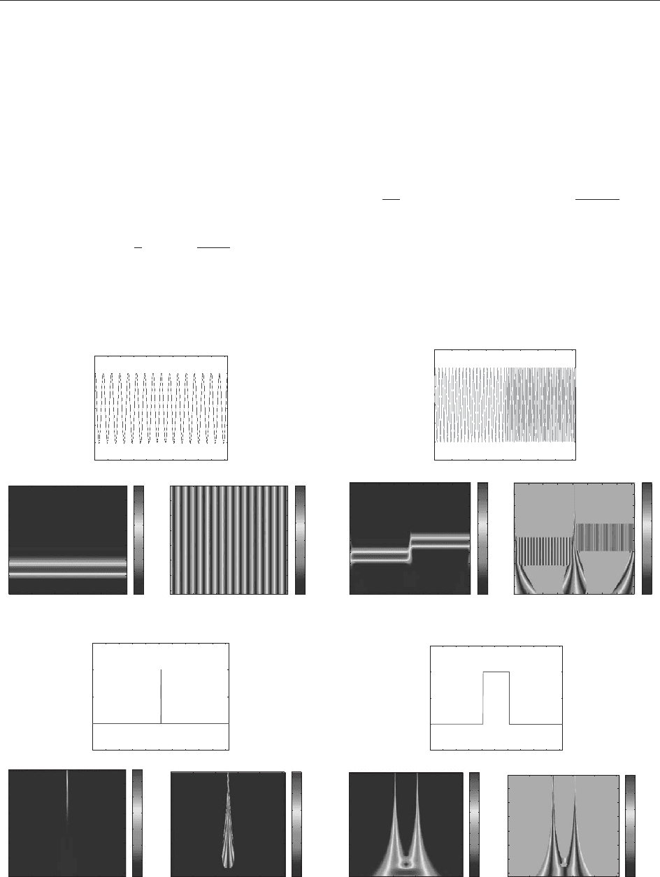
the four signals we plot the modulus and the phase

of the corresponding wavelet coefficients.

Higher Dimensions

The continuous wavelet transform can be extended to

higher dimensions in L

)indifferentways.Either

we define spherically symmetric wavelets by setting

(x) =

(jxj)forx 2 R

or we introduce in addition

to dilations a 2 R

and translations b 2R

also rota-

tions to define wavelets with a directional sensitivity. In

the two-dimensional case, we obtain for example,

a;b;

ðxÞ¼

1



x  b



½16

where a 2 R

, b 2 R

, and where R



is the rotation

matrix

cos  sin 

sin  cos 



½17

The analysis formula [8] then becomes

f ða; b;Þ¼

f ðxÞ



a;b;

ðxÞdx ½18

and for the corresponding inverse wavelet transform

[11] we obtain

f ðxÞ¼

2

f ða;b;Þ

a;b;

ðxÞ

dadbd

½19

Similar constructions can be made in dimensions

larger than 2 using n 1 angles of rotation.

0 100 200 300 400 500 600 700 800 900 1000

–1.5

–1

–0.5

0.5

1.5

Cosine

Two sines

0 500 1000 1500 2000 2500 3000 3500 4000

–1.5

–1

–0.5

0.5

1.5

0 100 200 300 400 500 600 700 800 900 1000

–0.5

0.5

Dirac

0 100 200 300 400 500 600 700 800 900 1000

–0.5

0.5

1.5

Characteristic function

Modulus of the wavelet coefficients Phase of the wavelet coefficients

0.1

0.2

0.3

0.4

0.5

0.6

0.7

0.8

0.9

200 400 600 800 1000

–3

–2

–1

200 400 600 800 1000

Modulus of the wavelet coefficients Phase of the wavelet coefficients

0.1

0.2

0.3

0.4

0.5

0.6

0.7

0.8

0.9

500 1000 1500 2000 2500 3000 3500 4000

–3

–2

–1

500 1000 1500 2000 2500 3000 3500 4000

Modulus of the wavelet coefficients

Phase of the wavelet coefficients

0.05

0.1

0.15

0.2

0.25

0.3

200 400 600 800 1000

0.5

1.5

2.5

200 400 600 800 1000

Modulus of the wavelet coefficients

0.02

0.04

0.06

0.08

0.1

0.12

0.14

0.16

0.18

200 400 600 800 1000

–3

–2

–1

200 400 600 800 1000

Phase of the wavelet coefficients

Figure 1 Examples of a one-dimensional continuous wavelet analysis using the complex-valued Morlet wavelet. Each subfigure

shows on the top the function to be analyzed and below (left) the modulus of its wavelet coefficients and below (right) the phase of its

wavelet coefficients.

428 Wavelets: Mathematical Theory

Discrete Wavelets

Frames

It is possible to obtain a discrete set of quasiortho-

gonal wavelets by sampling the scale and position

axes a, b. For the scale a we use a logarithmic

discretization: a is replaced by a

= a

j

, where a

the sampling rate of the log a axis (a

=( log a))

and where j 2 Z is the scale index. The position b is

discretized linearly: b is replaced by x

= ib

j

where b

is the sampling rate of the position axis at

the largest scale and where i 2 Z is the position

index. Note that the sampling rate of the position

varies with scale, that is, for finer scales (increasing j

and hence decreasing a

), the sampling rate

increases. Accordingly, we obtain the discrete wave-

lets (cf. Figure 2)

ðx

Þ¼a

1=2

 x



½20

and the corresponding discrete decomposition for-

mula is

¼h

; f i¼

1

f ðx



ðx

Þdx

½21

Furthermore, the wavelet coefficients satisfy the

following estimate:

Akf k



j;i

 Bkf k

½22

with frame bounds B  A > 0. In the case A = B we

have a tight frame.

The discrete reconstruction formula is

f ðxÞ¼C

j¼1

i¼1

ðxÞþRðxÞ½23

where C is a constant and R(x) is a residual, both

depending on the choice of the wavelet and the

sampling of the scale and position axes. For the parti-

cular choice a

= 2 (which corresponds to a scale

sampling by octaves) and b

= 1, we have the dyadic

sampling, for which there exist special wavelets

that

form an orthonormal basis of L

(R), that is, such that

;

i¼



½24

where  denotes the Kronecker symbol. This means

that the wavelets

are orthogonal with respect to

their translates by discrete steps 2

j

i and their dilates

by discrete steps 2

j

corresponding to octaves. In

this case, the recons truction formula is exact with

C = 1 and R = 0. Note that the discrete wavelet

transform has lost the invariance by translation and

dilation of the continuous one.

Orthogonal Wavelets and Multiresolution Analysis

The construction of orthogonal wavelet bases and the

associated fast numerical algorithm is based on the

mathematical concept of multiresolution analysis

(MRA). The underlying idea is to consider approx-

imations f

of the function f at different scales j.

The amount of information needed to go from a coarse

approximation f

to a finer resolution approximation

jþ1

is then described using orthogonal wavelets. The

orthogonal wavelet analysis can thus be interpreted as

decomposing the function into approximations of the

function at coarser and coarser scales (i.e., for

decreasing j), where the differences between the

approximations are encoded using wavelets.

The definition of the MRA was introduced by

Ste´phane Mallat in 1988 (Mallat 1989). This

technique constitutes a mathematical framework of

orthogonal wavelets and the related FWT.

A one-dimensional orthogonal MRA of L

(R)is

defined as a sequence of successive approximation

spaces V

, j 2 Z, which are closed imbedded subspaces

of L

(R). They verify the following conditions:

 V

jþ1

8j 2 Z ½25

[

j2Z

¼ L

ðRÞ½26

j2Z

¼f0g½27

f ðxÞ2V

, f ð2xÞ2V

jþ1

½28

3456 7

...

(a)

(b)

Figure 2 Orthogonal quintic spline wavelets

j, i

(x) = 2

j=2

x  i ) at different scales and positions: (a)

5, 6

(x),

6, 32

(x),

7, 108

(x), and (b) corresponding wavelet coefficients.

Wavelets: Mathematical Theory 429

A scaling function (x) is required to exist. Its

translates generate a basis in each V

, that is,

¼ spanf

i2Z

½29

where



ðxÞ¼2

j=2

ð2

x  iÞ; j; i 2 Z ½30

At a given scale j, this basis is orthonormal with respect

to its translates by steps i=2

but not to its dilates,

h

;

i¼

½31

The nestedness of the approximation spaces [28]

generated by the scaling function  implies that it

satisfies a refinement equation:



j1;i

ðxÞ¼

n¼1

n2i



ðxÞ½32

with the filter coefficients h

= h

, 

j1,0

i, which

determine the scaling function completely. In gen-

eral, only the filter coefficients h

are known and no

analytical exp ression of  is given. Equation [32]

implies that the approximation of a function at

coarser scale can be described by linear combina-

tions of the same function at finer scales.

The orthogonal projection of a function f 2 L

(R)

on V

is defined as

: f ! P

f ¼ f

½33

with

ðxÞ¼

k2Z

hf ;

i

ðxÞ½34

This coarse graining at a given scale J is done by

filtering the function with the scaling function .As

a filter, the scaling function  does not have

vanishing mean but is normalized so that

1

 (x)dx = 1.

As V

J1

is included in V

, we can define its

orthogonal complement space in V

¼ V

J1

 W

J1

½35

Correspondingly, the approximation of the func-

tion f at scale 2

J

, belonging to V

, can be

decomposed as a sum of orthogonal projections on

J1

and W

J1

, such that

f ¼ P

J1

f þ P

J1

f ½36

Based on the scaling function , one can construct a

function , the so-called mother wavelet, given by

the relation

ðxÞ¼

n2Z

n2i



j;n

ðxÞ½37

with g

= h

j1, 0

i, and where

(x) = 2

j=2

x  i), j, i 2 Z (cf. Figure 2). The filter coeffi-

cients g

can be computed from the filter coefficients

using the relation

¼ð1Þ

1n

½38

The translates and dilates of the wavelet

constitute orthonormal bases of the spaces W

¼ spanf

i2Z

½39

As in the continuous case, the wavelets have

vanishing mean, and also possibly vanishing higher-

order moments; therefore,

1

ðxÞdx ¼ 0 for m ¼ 0; ...; M  1 ½40

Let us now consider approximations of a function

f 2 L

(R) at two different scales j:



at scale j

ðxÞ¼

i¼1



ðxÞ½41



at scale j  1

j1

ðxÞ¼

i¼1

j1;i



j1;i

ðxÞ½42

with the scaling coefficients

¼hf ;

i½43

which correspond to local averages of the function

f at position i2

j

and at scale 2

j

The difference between the two approximations is

encoded by the wavelets

ðxÞf

j1

ðxÞ¼

i¼1

j1; i

j1;i

ðxÞ½44

with the wavelet coefficients

¼hf ;

i½45

which correspond to local differences of the function

at position (2 i þ 1)2

(jþ1)

between approximations

at scales 2

j

and 2

(jþ1)

Iterating the two-scale decomposition [44], any

function f 2 L

(R) can be expressed as a sum of a

coarse-scale approximation at a reference scale j

that we set to 0 here, and their successive

430 Wavelets: Mathematical Theory

differences. These details are needed to go from one

scale j to the next finer scale j þ 1 for

j = 0, ..., J  1,

f ðxÞ¼

i¼1

0;i



0;i

ðxÞþ

j¼0

i¼1

ðxÞ½46

For numerical applications, the sums in eqn [46]

have to be trunca ted in both scale j and position i.

The truncation in scale corresponds to a limitation

of f to a given finest scale J, which is in practice

imposed by the available sampling rate. Due to the

finite length of the available data, the sum over i

also becomes finite. The decomposition [46] is

orthogonal, as, by construction,

;

i¼



½47

;

i¼0 for j  j

½48

in addition to [31].

Fast Wavelet Transform

Starting with a funct ion f 2 L

(R) given at the finest

resolution 2

J

(i.e., we know f

2 V

and hence the

coefficients

for i 2 Z), the FWT computes its

wavelet coefficients

by decomposing successively

each approximation f

into a coarser scale approx-

imation f

J1

, plus the corresponding details which

are encoded by the wavelet coefficients. The

algorithm uses a cascade of discrete convolutions

with the low pass filter h

and the bandpass filter g

followed by downsampling, in which only one

coefficient out of two is retained. The direct wavelet

transform algorithm is



initialization

given f 2 L

ðRÞ and f

¼ f



for i 2 Z



decomposition

for j = J to 1, step 1, do

j1;i

n2Z

n2i

½49

j1;i

n2Z

n2i

½50

The inverse wavelet transform is based on

successive reconstructions of fine-scale approxima-

tions f

from coarser scale approximations f

j1

plus the differences between approximations at

scale j  1 and the finer scale j which are encoded

j1, i

. The algorithm uses a cascade of discrete

convolutions with the filters h

and g

, preceded by

upsampling which adds zeros in between two

successive coefficients.



reconstruction

for j = 1toJ, step 1, do

n¼1

i2n

j1;n

n¼1

i2n

j;n

½51

The FWT has been introduced by Ste´phane Mallat

in 1989. If the scaling functions (and wavelets) are

compactly supported, the filters h

and g

have only

a finite number of nonvanishing coefficients. In this

case, the numerical complexity of the FWT is O(N)

where N denotes the number of samples.

Choice of Wavelets

Orthogonal wavelets are typically defined by their

filter coefficients h

, since in general no analytic

expression for is available. In the following, we

give the filter coefficients of h

for some typical

orthogonal wavelets. The filter coefficients of g

can

be obtained using the quadrature relation between

the two filters [38].



Haar D1 (one vanishing moment):

¼ 1=

ﬃﬃﬃ

¼ 1=

ﬃﬃﬃ



Daubechies D2 (two vanishing moments):

¼ 0:482 962 913 145

¼ 0:836 516 303 736

¼ 0:224 143 868 042

¼0:129 409 522 551



Daubechies D3 (three vanishing moments):

¼ 0:332 670 552 950

¼ 0:806 891 509 311

¼ 0:459 877 502 118

¼0:135 011 020 010

¼0:085 441 273 882

¼ 0:035 226 291 882



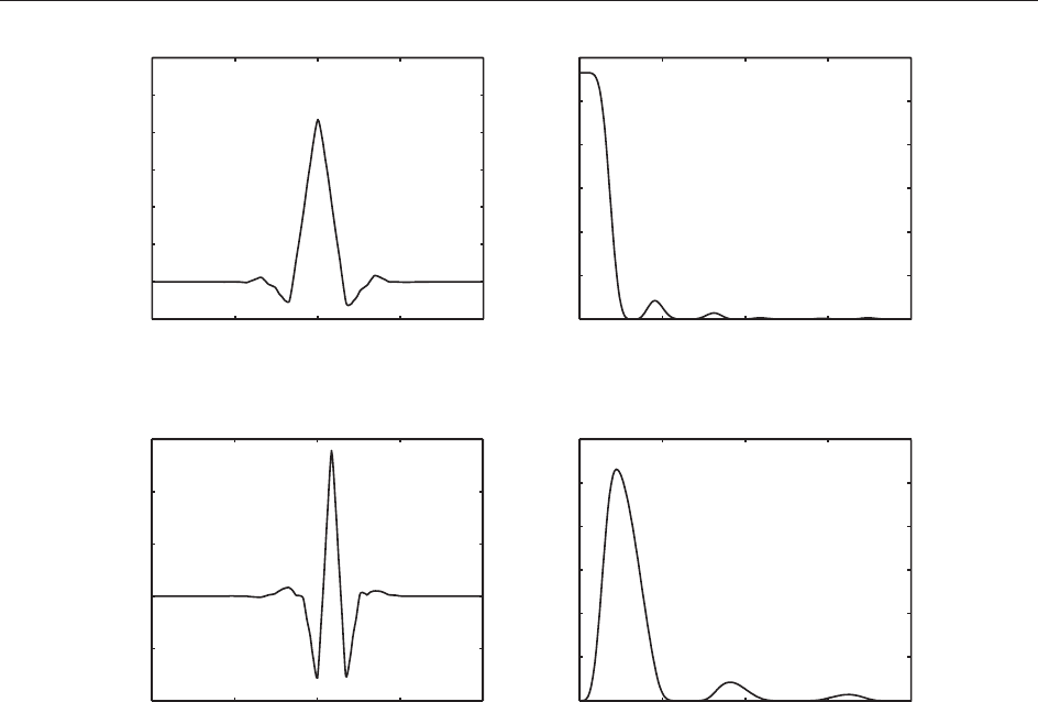
Coiflets C12 (four vanishing moments): the

wavelets and the corresponding scaling function

are shown in Figure 3.

Remarks The construction of orthogonal wavelets

in L

(R) can be modified to obtain wavelets on the

interval, that is, in L

([0, 1]). Therewith, boundary

wavelets are introduced, while in the interior of the

interval the wavelets are not modified.

Wavelets: Mathematical Theory 431

A periodic MRA of L

(T), wher e T = R=Z

denotes the torus, can also be constructed by

periodizing the wavelets in L

(R), using

per

ðxÞ¼

k2Z

ðx þ kÞ

Relaxing the condition of orthogonality allows

greater flexibility in the choice of the basis

functions. For example, biorthogonal wavelets can

be designed using differen t basis functions for

analysis (

) and synthesis (

) which are related

but no longer orthogonal. A couple of refinable

scaling functions (

, 

) with related wavelets

(

) which are by construction biorthogonal

generate a biorthogonal MRA V

, V

. From an

algorithmic point of view, only two different filter

couples (g

, h

) for the forward and (g

, h

) for the

backward FWT are used, without changing the

algorithm.

The multiresolution approach can be further

generalized, for samplings on nonequidistant

grids leading to the so-called second-generation

wavelets.

Higher Dimensions

The previously presented one-dimensional construc-

tion can be extended to higher dimensions. For

simplicity, we will consider only the two-

dimensional case, since higher dimensions can be

treated analogously.

Tensor product construction Having developed a

one-dimensional orthonormal basis

of L

(R), one

could use these functions as building blocks in

higher dimensions. One way of doing so is to take

the tensor product of two one-dimensional bases

and to define

ðx; yÞ¼

ðxÞ

ðyÞ½52

The resulting functions constitue an orthonormal

wavelet basis for L

). Each function f 2 L

)

can then be developed into

f ðx; yÞ¼

ðx; yÞ½53

with

, j

, i

= hf ,

, j

, i

i. However, in this basis

the two variables x and y are dilatated separately

1 0.5 0 0.5 1

0.05

0.1

0.15

0.2

0.25

0.3

0 50 100 150 200

(a)

1 0.5 0 0.5 1

0.2

0.1

0.2

0.3

0 50 100 150 200

(b)

Figure 3 Orthogonal wavelets Coiflet C12. (a) Scaling function (x ) (left) and j

(!)j. (b) Wavelet (x ) (left) and j

(!)j.

432 Wavelets: Mathematical Theory

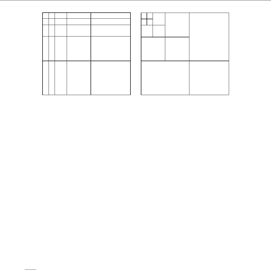
and therefore no longer form an MRA. This means

that the functions

, j

involve two scales, 2

and

, and each of the functions is essentially supported

on a rectangle with these side-lengths. Hence, the

decomposition is often called rectangular wavelet

decomposition (cf. Figure 4a). From the algorithmic

viewpoint, this is equivalent to applying the one-

dimensional wavelet transform to the rows and the

columns of a mat rix or a function. For some

applications, such a basis is advantageous, for others

not. Often the notion of a scale has a certain

meaning. For an application, one would like to have

a unique scale assigned to each basis function.

Multiresolution construction Another much more

interesting construction is the construction of a truly

two-dimensional MRA of L

). It can be obtained

through the tensor product of two one-di mensional

MRAs of L

(R). More precisely, one defines the

spaces V

, j 2 Z by

¼ V

 V

½54

and V

= span{

j, i

, i

(x, y) = 

j, i

(x)

j, i

(y), i

, i

2 Z}

fulfilling analogous properties as in the one-

dimensional case.

Likewise, we define the complement space W

be the orthogonal complement of V

in V

jþ1

, that is,

jþ1

¼ V

jþ1

 V

jþ1

¼ðV

 W

ÞðV

 W

Þ½55

¼V

 V

ððW

 V

ðV

 W

ÞðW

 W

ÞÞ ½56

¼ V

 W

½57

It follows that the orthogonal complement W

jþ1

 V

consists of three different types of func-

tions and is generated by three different wavelets

j;i

ðx; yÞ¼

j;i

ðxÞ

j;i

ðyÞ;"¼ 1



j;i

ðxÞ

j;i

ðyÞ;"¼ 2

j;i

ðxÞ

j;i

ðyÞ;"¼ 3

½58

Observe that here the scale parameter j simulta-

neously controls the dilatation in x and y. We recall

that in d dimensions this construction yields 2

1

types of wavelets spanning W

Using [58], each function f 2 L

) can be

developed into a multiresolution basis as

f ðx; yÞ¼

"¼1;2;3

j;i

ðx; yÞ½59

with

j, i

, i

=< f ,

j, i

, i

>. A schematic representa-

tion of the wavelet coefficients is sho wn in

Figure 4b. The algorithmic structure of the one-

dimensional transforms carries over to the two-

dimensional case by simple tensorization, that is,

applying the filters at each decom position step to

rows and columns.

Remark The described two-dimensional wavelets

and scaling functions are separable. This advantage is

the ease of generation starting from one-

dimensional MRAs. However, the main drawback

of this construction is that three wavelets are needed

to span the orthogonal complement space W

Another property should be mentioned. By construc-

tion, the wavelets are anisotropic, that is, horizontal,

diagonal, and vertical directions are preferre d.

Approximation Properties

Reproduction of Polynomials

A fundamental property of the MRA is the exact

reproduction of polynomials. The vanishing

moments of the wavele t , that is,

(x)dx = 0

...

... ...

...

–1, j

–1, i

, i

–1

, i

j, i

, i

j, i

, i

j, i

, i

–1

, i

–1

, i

, j

–1, i

, i

, j

, i

...

–1, j

, i

(a) (b)

Figure 4a Schematic representation of the 2D (b) wavelet transforms: (a) Tensor product construction and (b) 2D MRA.

Wavelets: Mathematical Theory 433

for m = 0, M  1, is equivalent to the fact that

polynomials up to degree M  1, can be expressed

exactly as a linear combination of scaling functions,

(x)=

n2Z

(xn) for m=0,M 1. This so-

called Strang–Fix condition proves that has M

vanishing moments if and only if any polynomial of

degree M 1 can be written as a linear combination

of scaling functions . Note that, as p

62L

(R), the

coefficients n

are not in l

(Z).

Regularity and Local Decay of Wavelet

Coefficients

The local or global regul arity of a function is closely

related to the decay of its wavelet coefficients. If a

function is locally in C

(R) (the space of s-times

continuously differentiable functions), it can be well

approximated locally by a Taylor series of degree s.

Consequently, its wavelet coefficients are small at

fine scales, as long as the wavelet has enough

vanishing moments. The decay of the coefficients

hence determines directly the error being made when

truncating a wavelet sum at some scale.

Depending on the type of norm used and whether

global or local characterization is concerned, various

relations of this kind have been developed. Let us

take as example the case of an -Lipschitz function.

Suppose f 2 L

(R), then for [a, b]  R the func-

tion f is -Lipschitz with 0 <<1 for any x

[a, b], that is, jf (x

þ h)  f (x

)jCjhj



,ifand

only if there exists a constant A such that j

j

j1=2

for any (j, i)withi=2

2 [a, b].

This shows the relation between the local reg-

ularity of a function and the decay of its wavelet

coefficients in scale.

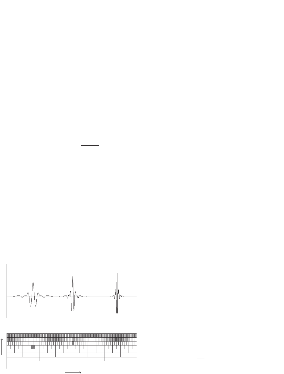
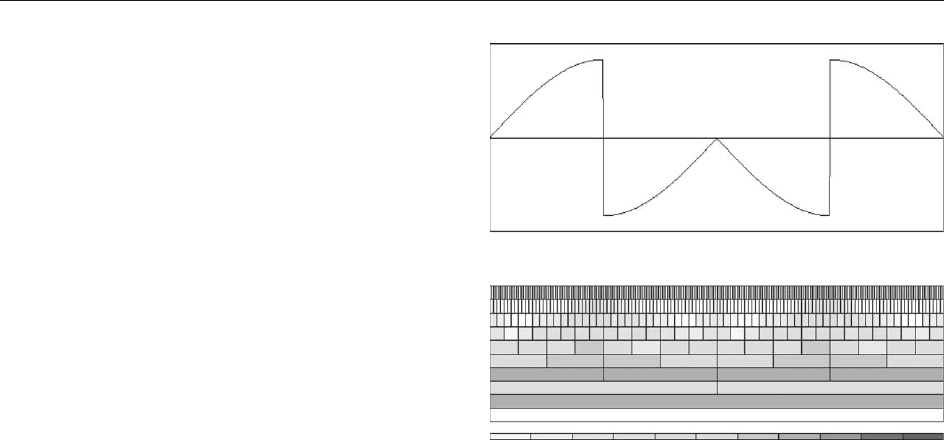
Example To illustrate the local decay of the

wavelet coefficients, we consider in Figure 5 the

function f (x) = sin (2x) for x  1=4 and x  3=4

and f (x) = sin (2x) for 1=4 < x < 3=4. The corre-

sponding wavelet coefficients for quintic spline

wavelets are plotted in logarithmic scale. The

wavelet coefficients show that only in a local region

around singularities the fine-scale coefficients are

significant.

Linear Approximation

The exact reproduction of polynomials can be used

to derive error estimates for the approximation of a

function f at a given scale, which corresponds to

linear approximation. We consider f belonging to

the Sobolev space W

s, p

), that is, the weak

derivatives of f up to order s belong to L

). The

linear approximation of f at scale J, corresponding

to the projection of f onto V

, is then given by

ðxÞ¼

J1

j¼0

i2Z

j;i

ðxÞ½60

The approximation error can be estimated by

kf  f

< C2

J minðs;mÞ=d

½61

where s denotes the smoothness of the function in

, d the space dimension, and m the number of

vanishing moments of the wavelet . In the case of

poor global regularity of f, that is, for small s,a

large number of scales J is needed to get a good

approximation of f.

In Figure 6, we plot the linear approximation of

the function f shown in Figure 5. The function f

reconstructed using wavelet coefficients up to scale

J  1 = 5, so that in total only 64 out of 512

coefficients are retained. We observe an oscillating

behavior of f

near the discontinuities of f which

dominates the approximation error.

Nonlinear Approximation

Retaining the N largest wavelet coefficients in the

wavelet expansion of f in [46], without imposing

any a priori cutoff scale, yields the best N-term

approximation f

. In contrast to the linear approx-

imation [60], it is called nonlinear approximation,

since the choice of the retained coefficients depends

–4.00E + 00 Logarithm 1.00E + 00

(a)

(b)

Figure 5 Orthogonal wavelet decomposition using quintic

spline wavelets: (a) function f (x ) = sin (2x) for x  1=4 and x 

3=4 and f (x )= sin(2x) for 1=4 < x < 3=4 sampled on a grid

=i=2

,i = 0,...,2

1 with J =9 and (b) corresponding wavelet

coefficients log

j, i

j for i = 0,...,2

1 and j =0,...,J 1.

434 Wavelets: Mathematical Theory

on the function f. The mathematical theory has been

formalized by Cohen, Dahmen, and De Vore.

The nonlinear approximation of the function f can

then be written as

ðxÞ¼

ðj;iÞ2

j;i

ðxÞ½62

where 

denotes the ensemble of all multi-indices

 = (j, i), indexing the N largest coefficients (mea-

sured in the l

norm),



¼f

;k ¼1; Njk



> k



8 2g½63

with ={= (j,i),j 0,i 2Z}. The nonlinear

approximation leads to the following error estimate:

kf  f

< CN

s=d

½64

where s denotes the smoothness of f in the larger

space L

) with

which corresponds to the Sobolev embedding line

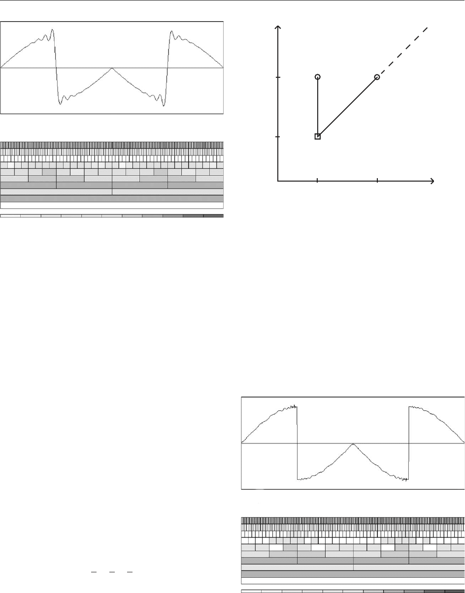
(Figure 7). This estimate shows that the nonlinear

approximation converges faster than the linear one,

if f has a larger regularity in L

, that is, f 2 W

s, q

), which is for example the case for functions

with isolated singularities and for small q.

In Figure 8, we plot the nonlinear approximation

of the function f shown in Figure 5. The function f

is reconstructed using the strongest 64 wavelet

coefficients out of 512 coefficients. Compared to

the linear approximation (cf. Figure 6), the oscilla-

tions around the discontinuities disappear and the

approximation error is reduced while using the same

number of coefficients.

Compression and Preconditioning of Operators

The nonlinear approximation of functions can be

extended to certain operators leading to an efficient

(IR

)

(IR

)

1/p

1/q

= 1/p + t /d

Embedding

Linear approx.

O(N

–t /d

)

Nonlinear approx.

O(N

–t /d

)

s,p

(IR

)

Figure 7 Schematic representation of linear and nonlinear

approximation.

–4.00E + 00 Logarithm 1.00E + 00

(a)

(b)

Figure 6 (a) Linear approximation f

of the function f in

Figure 5 for J = 6, reconstructed from 64 wavelet coefficients

using quintic splines wavelets and (b) corresponding wavelet

coefficients log

j, i

j for i = 0, ...,2

 1 and j = 0, ..., J  1.

Note that the coefficients for J > 5 have been set to zero.

–4.00E + 00 Logarithm 1.00E + 00

(a)

(b)

Figure 8 (a) Nonlinear approximation f

of the function f in

Figure 5 reconstructed from the 64 largest wavelet coefficients

using quintic splines wavelets, (b) retained wavelet coefficients

log

j, i

j for i = 0, ...,2

 1 and j = 0, ..., J  1.

Wavelets: Mathematical Theory 435

representation in wavelet space, that is, to sparse

matrices. For integral operators, for example,

Calderon–Zygmund operators T on R defined by

Tf ðxÞ¼

Kðx; yÞf ðyÞdy ½65

where the kernel k satisfies

jkðx; y; Þj 

jx  yj

and

kðx; yÞ



kðx; y; Þ





jx  yj

their wavelet representation hT

j, i

, i

i is sparse

and a large number of weak coefficients can be

suppressed by simple thresholding of the matrix

entries while controlling the precision. The resulting

numerical scheme is called BCR algorithm and is

due to Beylkin et al. (1991).

The characterization of funct ion spaces by the

decay of the wavelet coefficients and the corre-

sponding norm equiva lences can be used for

diagonal preconditioning of integral or differential

operators which leads to matrices with uniformly

bounded condition numbers. For elliptic differential

operators, for example, the Laplace operator r

the

norm equivalence kr

f k’k2

k can be used for

preconditioning the matrix hr

j, i

, i

i by a simple

diagonal scaling with 2

2j

to obtain a uniformly

bounded condition number. For further details, we

refer to the book of Cohen (2000).

Wavelet Denoising

We consider a function f which is corrupted by a

Gaussian white noise n 2N(0, 

). The noise is

spread over all wavelet coeffic ients



, while,

typically, the original function f is deter mined by

only few significant wavelet coefficients. The aim is

then to reconstruct the function f from the observed

noisy signal s = f þ n.

The principle of the wavelet denoising can be

summarized in the following procedure:



Decomposition. Compute the wavelet coefficients



using the FWT.



Thresholding. Apply the thresholding function 

to the wavelet coefficients



, thus reduci ng the

relative impo rtance of the coefficients with small

absolute value.



Reconstruction. Reconstr uct a denoised version s

from the thresholded wavelet coefficients using

the fast inverse wavelet transform.

The thresholding parameter " depends on the

variance of the noise and on the sample size N.

The thresholding function  we consider corre-

sponds to hard thresholding:



ðaÞ¼

a if jaj >"

0ifjaj"



½66

Donoho and Johnstone (1994) have shown that

there exists an optimal " for which the relative

quadratic error between the signal s and its

estimator s

is close to the minimax error for all

signals s 2H, where H belongs to a wide class of

function spaces, including Ho¨ lder and Besov spaces.

They showed using the threshold

¼ 

ﬃﬃﬃﬃﬃﬃﬃﬃﬃﬃﬃﬃﬃ

2lnN

½67

yields an error which is close to the minimum error.

The threshold "

depends only on the sampling N

and on the variance of the noise 

; hence, it is

called universal threshold. How ever, in many

applications, 

is unknown and has to be estimated

from the available noisy data s. For this, the present

authors have developed an iterative algorithm (see

Azzolini et al. (2005)), which is sketched in the

following:

1. Initialization

(a) given s

, k = 0, ..., N  1. Set i = 0 and com-

pute the FWT of s to obtain



;

(b) compute the variance 

of s as a rough

estimate of the variance of n and compute the

corresponding threshold "

= (2 ln N

)

1=2

;

noise N

noise

= N.

2. Main loop repeat

(a) set N

noise

= N

noise

and count the wavelet

coefficients N

noise

with modulus smaller

than "

;

(b) compute the new variance 

iþ1

from the

wavelet coefficients whose modulus is smal-

ler than "

and the new threshold "

iþ1

(2( ln N)

iþ1

)

1=2

;

noise

==N

noise

3. Final step

(a) compute s

from the coefficients with mod-

ulus larger than "

using the inverse FWT.

Example To illustrate the properties of the denoising

algorithm, we apply it to a one-dimensional test signal.

We construct a noisy signal s by superposing a

Gaussian white noise, with zero mean and variance



= 1, to a function f,normalizedsuchthat

((1=N)

)

1=2

= 10. The number of samples is

436 Wavelets: Mathematical Theory

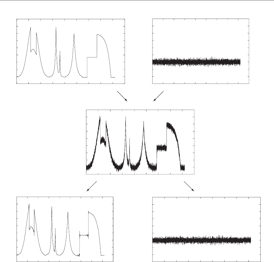
N = 8192. Figure 9a shows the function f together

with the noise n; Figure 9b shows the constructed

noisy signal s and Figure 9c shows the wavelet

denoised signal s

together with the extracted noise.

Acknowledgments

Marie Farge thankfully acknowledges Trinity Col-

lege, Cambridge, UK, and CIRM, Marseille, France,

for support while writing this paper. The authors also

thank Barbara Burke for kindly revising their English.

See also: Coherent States; Fractal Dimensions in

Dynamics; Homeomorphisms and Diffeomorphisms of

the Circle; Image Processing: Mathematics; Wavelets:

Application to Turbulence; Wavelets: Applications.