Francoise J.-P., Naber G.L., Tsun T.S. (editors) Encyclopedia of Mathematical Physics

Подождите немного. Документ загружается.

operator, which resolves one problem of the one-particle

theory. However, q(K) is not bounded from below, and

thus 

(0)



is not yet the physical representation.

The physical representation can be constructed

using the operators

T ¼

ﬃﬃﬃ

1=2

1=2

1=2

1=2



; F ¼

0 1



½53

(for simplicity, we restrict ourselves to the case C = 0

and B > 0; we use the calculus of self-adjoint operators

here) with the following remarkable properties:

1

¼ JT



TKT

1

B 0

0 B





½54

One can check that

ðf Þ

ðTf Þ;

ðf Þ ðT

1

f Þ½55

is a quasifree representation 



of A



(h) with



= (1  F)=2. With that the construction of

q and

Q is very similar to the fermion case described

above (the crucial simplification is that

K and F now

are diagonal). In particular,

q(K) is a non-negative

operator with the ground state , and

q(A) and

Q(U) are self-adjoint and unitary for every one-

particle observable A and transformation U, respec-

tively. One also gets relations as in [43] and [46].

Further Reading

Carey AL and Ruijsenaars SNM (1987) On fermion gauge

groups, current algebras and Kac–Moody algebras. Acta

Applicandae Mathematicae 10: 1–86.

DeWitt B (2003) The Global Approach to Quantum Field

Theory, International Series of Monographs on Physics, vols.

1 and 2, p. 114. New York: Oxford University Press.

Gracia-Bondı´a JM, Va´rilly JC, and Figueroa H (2001) Elements

of Noncommutative Geometry, Birkha¨ user Advanced Texts:

Basel Textbooks. Boston: Birkha¨user.

Grosse H and Langmann E (1992) A superversion of quasifree second

quantization. Journal of Mathematical Physics 33: 1032–1046.

Kac VG and Raina AK (1987) Bombay Lectures on Highest

Weight Representations of Infinite-Dimensional Lie Algebras,

Bosons and Fermions in External Fields 325

Advanced Series in Mathematical Physics, vol. 2. Teaneck:

World Scientific Publishing.

Langmann E (1994) Cocycles for boson and fermion Bogoliubov

transformations. Journal of Mathematical Physics 96–112.

Langmann E (1996) Quantum gauge theories and noncommuta-

tive geometry. Acta Physica Polonica B 27: 2477–2496.

Mickelsson J (1989) Current Algebras and Groups, Plenum

Monographs in Nonlinear Physics. New York: Plenum Press.

Rafelski J, Fulcher LP, and Klein A (1978) Fermions and bosons

interacting with arbitrary strong external fields. Physics

Reports 38: 227–361.

Reed M and Simon B (1975) Methods of Modern Mathematical

Physics. II. Fourier Analysis, Self-Adjointness. New York:

Academic Press.

Ruijsenaars SNM (1977) On Bogoliubov transformations for

systems of relativistic charged particles. Journal of Mathema-

tical Physics 18: 517–526.

Weinberg S (1995) The Quantum Theory of Fields,vol.I(English

summary) Foundations. Cambridge: Cambridge University Press.

Boundaries for Spacetimes

S G Harris, St. Louis University, St. Louis, MO, USA

Introduction

There is a common practice in mathematics of placing a

boundary on an object which may not appear to come

naturally equipped with one; this is often thought of as

adding ideal points to the object. Perhaps the most

famous example is the addition of a single ‘‘point at

infinity’’ to the complex plane, resulting in the Riemann

sphere: this is a boundary point in the sense of providing

an ideal endpoint for lines and other endless curves in

the plane. Often, there is more than one reasonable way

to construct a boundary for a given object, depending

on the intent; for instance, the plane is sometimes

equipped, not with a single point at infinity, but with a

circle at infinity, resulting in a space homeomorphic to a

closed disk. Both these boundaries on the plane have

useful but different things to tell us about the nature of

the plane; the common feature is that, by bringing the

infinite reach of the plane within the confines of a more

finite object, we are better able to grasp the behavior of

the original object.

The general usefulness of the construction of

boundaries for an object is to allow behavior of

structures in the ‘‘completed’’ object to aid in

visualization of behavior in the original object,

such as by providing a degree of measurement or

other classification of processes at infinity. This

utility has not been overlooked for spacetimes. A

variety of purposes may be served by various

boundary construction methods: providing a locale

for singularities (as the spacetime itself is modeled

by a smooth manifold with a smooth metric, free of

singular points); providing a platform from which to

measure global properties such as total energy or

angular momentum; displaying in finite form the

causal structure at infinity; or providing a compact

(or quasicompact) topological envelope for the

spacetime while preserving the causal structure.

This article will consider several of the methods

that have been used or proposed for constructing

boundaries for spacetimes, ranging from the ad hoc

(but practical) to the universal. Perhaps the

simplest way to classify these methods is into

those which employ or analyze embeddings of the

spacetime in question and those that do not.

Boundaries from Embeddings

General

The simplest and most common method of construct-

ing a boundary for a spacetime M is to find a suitable

manifold N (of the same dimension) and an appro-

priate map  : M ! N which is a topological embed-

ding, that is, a homeomorphism onto its image (M).

We can consider



, the closure of (M)inN,asthe

-completion of M,and@



(M) =



 (M)asthe

-boundary. Typically, this embedding is chosen in

such a way that curves of interest in M –suchas

timelike or null geodesics or causal curves of bounded

acceleration – which have no endpoints in M, do have

endpoints in @



(M); in other words, if c : [0, 1) ! M is

such a curve of interest, then lim

t!1

(c(t)) exists in N.

The common practice, initiated by Penrose in

1967, is to choose N to be another spacetime –

often called the unphysical spacetime, while M is

considered the spacetime of physical interest – and to

require the embedding  to be a conformal mapping,

that is,  carries the spacetime metric in M to a scalar

multiple of the spacetime metric in N. As conformal

maps preserve the local causal structure, leaving

unchanged the notions of timelike curve or null

curve, this means that



inherits from N a causal

structure which, locally, is an extension of that of M.

This allows us to speak of causal relationships within



, closely related to those in M.

Minkowski Space

The prototypical example is the conformal embedding

of Minkowski space into the Einstein static spacetime.

326 Boundaries for Spacetimes

Let R

denote Euclidean n-space, S

the unit

n-sphere, and L

Minkowski n-space, that is, R

with

metric ds

= dx

þþdx

n1

 dt

(so L

n1

 L

). The n-dimensional Einstein static space-

time is the product spacetime E

= S

n1

 L

.Con-

sider S

n1

as embedded in R

= R

n1

 R

. Then the

conformal embedding is  : L

! E

,expressedas

 : R

n1

 L

! S

n1

 L

 R

n1

 R

 L

given

by (x, t) = ((x=j xj)sin ,cos, ), where  = tan

1

(t þjxj)  tan

1

(t jxj)and = tan

1

(t þjxj) þ

tan

1

(t jxj). The boundary @



)consistsofthe

following: the points { þ  = ;0 < }, composed

of an S

n2

of null lines coming together at the point

= (0,1,); a similar cone of null lines {   = ;

  <0} with vertex at i



= (0,1, ); and a single

limit-point for both cones at i

= (0, 1, 0). The >0

null cone is called I

(the letter is read ‘‘scri’’ for

‘‘script-I’’), its counterpart I



(Figures 1 and 2). As all

future-directed timelike geodesics in L

have i

as an

endpoint in E

, i

is called future-timelike infinity;

similarly, i



is past-timelike infinity. Every future-

directed null geodesic ends up on I

, which is thus

termed future-null infinity, and I



is past-null infinity.

All spacelike geodesics come to i

, spacelike infinity.

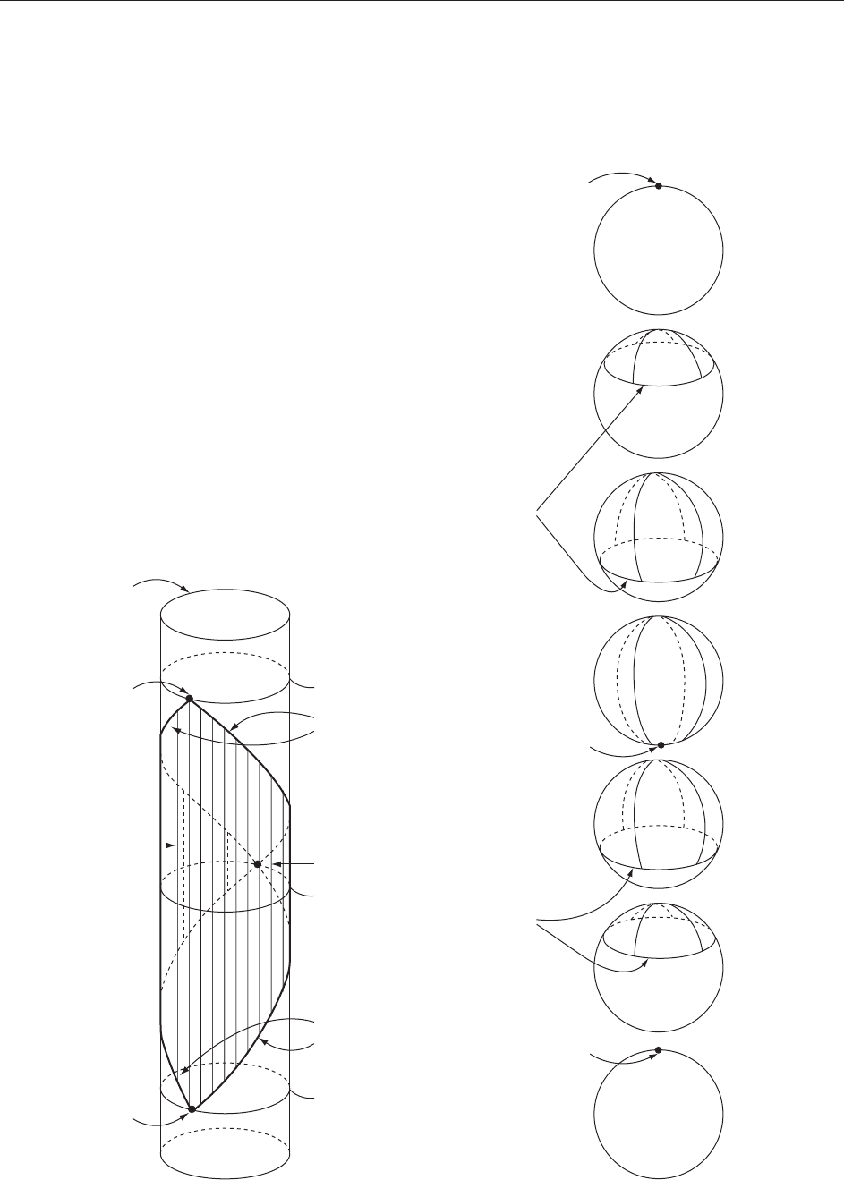
For n = 2, this picture produces the familiar

diamond representation of L

(Figure 3): as E

easily unrolled into another copy of L

(metric

–

ᑣ

Image of L

ᑣ

–

τ = –

τ = π

τ = 0

Figure 1 L

conformally embedded in E

= S

 L

ᑣ

–

ᑣ

τ = π

= 0

= –

Figure 2 L

conformally embedded in E

= S

 L

Boundaries for Spacetimes 327

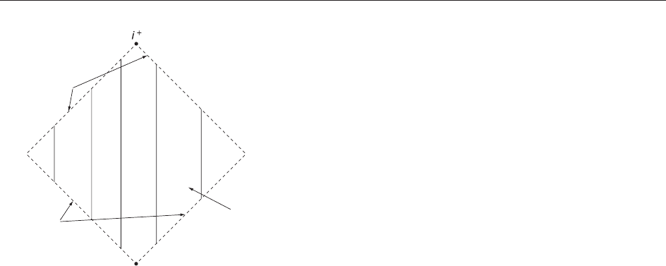
d

 d

), this means that (L

) is the region jjþ

jj < in L

; timelike curves and null geodesics in

the original L

are the same as in (L

), and their

endpoints in the boundary of the diamond are

evident. For higher dimensions, the picture is not as

visually obvious, since E

cannot be unrolled; but the

principle of reading the causal structure at infinity of

via its boundary points in E

remains the same.

Conformal Embeddings

There have been various formulations designed to

emulate the conformal mapping of L

with respect to

spacetimes, which are, in some sense, asymptotically

like Minkowski space being conformally mapped into

larger spacetimes. A spacetime M with metric g is

called asymptotically simple or (alternatively) asymp-

totically flat if there is a spacetime N with metric h,

an embedding  : M ! N, and a scalar function 

defined on N with 



h = (  )

g (i.e.,  is

conformal with 

the conformal factor) and =0

on @



(M), d 6¼ 0on@



(M), and various other

restrictions on , depending on the intent. One can

define asymptotic symmetries of M by means of

motions within @



(M), leading to notions of global

energy and angular momentum (see Hawking and

Ellis (1973) and Wald (1984) for details).

Classifications of Embeddings

As a general rule, there is no uniqueness in the

choice of an embedding  for a spacetime M to

construct a boundary, nor in the topology of the

resulting boundary @



(M), or even of which curves

of interest end up having endpoints in the boundary.

In an attempt to categorize which embeddings yield

equivalent results and what sort of results there are

in terms of endpoints of curves, Scott and Szekeres

(1994) formulated what they called the abstract

boundary of a spacetime. This depends on a choice

of class of ‘‘interesting’’ curves, each characterizable

as having either infinite or finite parameter length;

typical choices for this class would be timelike

geodesics or causal geodesics or timelike curves of

bounded acceleration. For instance, a boundary

point may be said to represent a singularity with

respect to the chosen class of curves if it is the

endpoint of one such curve with finite parameter

length; nonsingular points are points at infinity.

These classifications do not require conformal

embeddings, nor even that the target of the embed-

dings be spacetimes; they accommodate boundaries

of a far more general type than Penrose’s notion

stemming from conformal embeddings.

A somewhat different study of boundaries from

embeddings has been formulated by Garcı´a-Parrado

and Senovilla (2003), classifying points at infinity and

singularities in @



(M) for embeddings  : M ! N in

which N is a spacetime,  preserves the chronology

relation , and there is also a diffeomorphism

: (M) ! N which again preserves  (the chronol-

ogy relation in a spacetime is defined thus: x  y if

and only if there is a future-directed timelike curve

from x to y). This scheme applies more generally than

to conformal embeddings, but the requirement for

chronology-preserving maps in both directions guar-

antees a strong sensitivity to causality; it amounts to a

mild extension of Penrose’s notion that is often much

easier to construct.

Universal Constructions

B-Boundary

Attempts have been made to formulate boundary

concepts specifically for defining singularities as

ideal endpoints for finite-length geodesics. The

most complete venture in this direction is the

b-boundary (‘‘b’’ for ‘‘bundle’’) of Schmidt (Hawking

and Ellis 1973, pp. 276–284). This is a formulation

that takes note only of the connection in the linear

frames bundle L(M) of a spacetime M (or of any

manifold with a linear connection, metric or other-

wise); in other words, it takes no particular note of

the spacetime metric or even of the causal structure of

the spacetime, but only of the notion of parallel

translation of tangent vectors along curves. Parallel

translation of a frame (a basis for the tangent space)

along a curve is used to obtain an ad hoc length for

the curve by treating the translated frame as positive-

definite orthonormal at each point; whether this

length is finite or infinite is independent of the choice

of the original frame. The Schmidt construction

–

ᑣ

–

Image of L

Unrolled E

Figure 3 L

conformally embedded in unrolled E

, i.e.,

 L

= L

328 Boundaries for Spacetimes

defines a boundary on M which gives an endpoint for

each curve, endless in M, which is finite in that sense:

Select a positive-definite metric on L(M ), give it a

boundary by means of Cauchy completion, and then

take the appropriate quotient by the bundle group.

This has an appealing universality of application, but

the problems of putting it into practice are quite

formidable. Also, the fact that it takes no special note

of the spacetime character of M suggests that it may

not be of particular utility for physical insights.

Causal Boundary: Basics

In 1972 Geroch, Kronheimer, and Penrose (GKP)

formulated a notion of boundary – the causal

boundary – that is specifically adapted to the causal

character of a spacetime M; indeed, it is defined in

such a way that one need know only the chronology

relation  on M without any further reference to

the metric (another way of saying this is that the

causal boundary is conformally invariant). Like

Schmidt’s b-boundary, the causal boundary is a

universal construction, not depending on any extra-

neous choices; however, although it has an obvious

clarity in its causal structure, there are subtleties in

the choice of an appropriate topology which are

perhaps not yet fully resolved. As this boundary

construction appears to embody the best hopes for a

practical universal construction, it is detailed here in

some depth.

The causal boundary construction applies only to

strongly causal spacetimes; essentially, this means

that the local causal structure at each point is

exactly reflective of the global causal structure.

The basic construction of the causal boundary of

a spacetime M starts with two separate parts: the

future and past (pre-)boundaries of M, intended as

yielding endpoints for, respectively, future- and past-

endless causal curves. Part of the difficulty of the

causal boundary is knowing how best to meld these

two into one; currently, there are several answers to

this conundrum.

The elements of the future causal boundary of M

are defined in terms of the past-set operator I



. For

a point x 2 M, the past of x is I



(x) = {y jy  x}; for

a set A  M, I



[A] =

x2A



(x). A set P  M is

called a past set if I



[P] = P; anything of the form

P = I



[A] is a past set, and all past sets have this

form. A past set P is an indecomposable past set (IP)

if P cannot be written as P

[ P

for past sets which

are proper subsets P

( P. IPs come in exactly two

varieties: pointlike IPs (PIPs), of the form I



(x)

(Figure 4), and terminal IPs (TIPs), of the form I



[c]

for c a future-endless causal curve (Figure 5). (Of

course, any I



(x) can also be expressed as I



[c] for c

a causal curve ending at x.) The future causal

boundary of M,

@(M), consists of all the TIPs of M;

the future causal completion of M is

M =

@(M) [ M.

But that is just a set; the causal structure of M needs

to be extended to

For any x 2 M and P 2

@(M), set x  P if and

only if x 2 P; set P  x if and only if P  I



(y) for

some y  x (y 2 M); and for P and Q in

@(M), set

P  Q if and only if P  I



(y) for some y 2 Q.

If we consider this an extension of the  relation on

M, then we end up with a relation which, like that

on M, is transitive and antireflexive. Furthermore, it

has the property that for all ,  2

M,    if and

only if for some x 2 M,   x  . (One can also

amend the chronology relation within M to be more

like the definition in the extension; that is not of

major import.)

We can also extend the causality relation  on M

to one on

M (in M, x  y if there is a future-directed

Figure 4 PIP P = I



(x).

Figure 5 TIP P = I



Boundaries for Spacetimes 329

causal curve from x to y ): for x 2 M and P, Q 2

@(M), x  P for I



(x)  P, P  x for P  I



(x), and

P  Q for P  Q.

The intent is to have the elements of

@(M) provide

future endpoints for future-endless causal curves in

M; in particular, we want two such curves, c

and

, to be assigned the same future endpoint precisely

when I



] = I



]. This is accomplished by the

simple expedient of defining the future endpoint of a

future-endless causal curve c to be P = I



[c]. We do

not have a topology on

M as yet, but it is worth

noting that if P is the assigned future endpoint of c,

then I



(P) = I



[c]; this is at least the correct causal

behavior for a putative future endpoint of c.

We can perform all the operations above in the

time-dual manner, obtaining the past causal bound-

ary



@(M), consisting of terminal indecomposable

future sets (TIFs), and the past causal completion



M =



@(M) [ M. The full causal boundary of M

consists of the union of

@(M) with



@(M) with some

sort of identifications to be made.

As an example of the need for identifications,

consider M to be L

with a closed timelike line

segment deleted, say M = L

 {(0, t) j0  t  1}.

For

@(M), we have first the boundary elements at

infinity: the TIP i

= M (the past of the positive time

axis) and the set of TIPs making up I

(the pasts of

null lines going out to infinity in L

); and then, the

boundary elements coming from the deleted points:

for each t with 0 < t  1, two IPs emanating from

(0, t), that is, P

, the past of the null line going

pastwards from (0, t) toward x > 0, and P



, the past

of the null line going pastwards from (0, t) toward

x < 0; and P

, emanating from (0, 0), that is, the

past of the negative time axis. Similarly,



@(M)

consists of i



, I



, TIFs F

and F



emanating from

(0, t) for 0  t < 1, and the TIF F

emanating from

(0, 1). We probably want to make at least the

following identifications for each t with 0 < t < 1,

 F

and P



 F



; P

 F

 P



; and F



 F



. This results in a two-sided replacement

for the deleted segment; for some purposes, it might

be deemed desirable to identify the two sides as one,

but a universal boundary is probably a good idea,

leaving further identifications as optional quotients

of the universal object.

How best to define the appropriate identifications

in general is a matter of some controversy. GKP

defined a somewhat complicated topology on



M =

@(M) [



@(M) [ M, then used an identification

intended to result in a Hausdorff space. There are

significant problems with this approach in some

outre´ spacetimes, as pointed out by Budic and Sachs

(1974) and Szabados (1989), both of whom recom-

mended a different set of identifications. But what is

of more concern is that the topology prescribed by

GKP is not what might be expected in even the

simplest of cases, for example, Minkowski space:

needs no identifications among boundary points (no

matter whose identification procedure is followed).

The GKP topology on

,restrictedto

@(L

), is not

that of a cone (S

n2

 R

with a point added), as is

the case for I

in the conformal embedding into E

;

but, instead, each null line in

@(L

) (not including i

)

is an open set, and i

has no neighborhood in

@(L

)

save for the entire boundary. This is a topology

bearing no relation at all to that of any embedding.

Future Causal Boundary

Construction An alternative approach, initiated by

Harris (1998), is to forego the full causal boundary

and concentrate only on

M and



M separately. There

is an advantage to this in that the process of future

causal completion – that is to say, forming

M from

M – can be made functorial in an appropriate

category of ‘‘chronological sets’’: a set X with a

relation  which is transitive and antireflexive such

that it possesses a countable subset S which is

‘‘chronologically dense,’’ that is, for any x, y 2 X,

there is some s 2 S with x  s  y. Any strongly

causal spacetime M is a chronological set, as is

The entire construction of the future causal bound-

ary works just as well for a chronological set. The

role of a timelike curve in a chronological set is

taken by a future chain: a sequence c = {x

} with

 x

nþ1

for all n.Foranyfuturechainc, I



[c]isan

IP, and any IP can be so expressed; but unlike in

spacetimes, I



(x) may or may not be an IP for x 2 X.

Then,

X is always future complete in the sense that

for any future chain c in

X, there is an element  2

with I



() = I



[c]: for instance, if the chain c lies in

X but there is no x 2 X with I



(x) = I



[c], just let

 = I



[c], which is an element of

@(X). This yields a

functor of future completion from the category of

chronological sets to the category of future-complete

chronological sets, and the embedding X !

X is a

universal object in the sense of the category theory;

this implies that it is categorically unique and is the

minimal future-completion process.

However, it is crucial to have more than the

chronology relation operating in what is to be a

boundary; topology of some sort is needed. This is

accomplished by defining what might be called the

future-chronological topology for any chronological

set – including for

M when M is a strongly causal

spacetime. This topology is defined by means of a

limit-operator

L on sequences: if X is the chron-

ological set, then for any sequence of points  = {x

}

in X,

L() denotes a subset of X which is the set of

330 Boundaries for Spacetimes

limits of . It is explicitly recognized that there may

be more than one limit of a sequence, as the space

may not be Hausdorff; no attempt is made to

remove any non-Hausdorffness, as this is viewed as

giving important information on how, possibly,

two points in the future causal boundary represent

very similar and yet not identical pieces of

information about the causal structure at infinity.

Once the limit operator is in place, the actual

topology on X is defined thus: a subset A  X is

said to be closed if and only if for any sequence

  A,

L()  A (and open sets are complements of

closed sets). This yields the elements of

L()as

topological limits of .

The definition of

L is simplest when X has the

property that I



(x) is an IP for any x 2 X; as this is

true for X being either a spacetime M or the future

causal completion

M of a spacetime, the discussion

here is restricted to this situation. Let us also make

the common assumption that X is past-distinguishing,

that is, I



(x) = I



(y)impliesx = y.

Let  = {x

} be a sequence of points in a past-

distinguishing chronological set X in which the past

of any point is an IP. Then

L() consists of those

points x for which (see Figures 6 and 7)

1. for all y 2 I



(x), for n sufficiently large, y  x

and

2. for any IP P ) I



(x), there is some z 2 P such that

for n sufficiently large, z 6 x

Then the future-chronological topology on X has

these features:

1. It is a T

topology, that is, points are closed.

2. If I



(x) = I



[c] for a future chain c = {x

}, then x

is a topological limit of the sequence {x

3. If X = M, a strongly causal spacetime, then the

future-chronological topology is precisely the

manifold topology.

4. If X =

M, the future causal completion of a

strongly causal spacetime M, then the induced

topology on M is the manifold topology,

@(M)is

a closed subset of

M, and M is dense in

M. As per

property (2), for any future-endless causal curve c

in M, the point I



[c]in

@(M) is the topological

endpoint of c in

5. If X =

,thenX is homeomorphic to the conformal

image of L

in E

together with I

and i

;in

particular,

@(L

) has the topology of a cone.

Examples The future causal boundary with the

future-chronological topology can be calculated

with a fair degree of success. For instance, if M

is conformal to a simple product spacetime Q  L

(Q a Riemannian manifold), then

@(M)ismuch

@(L

) in that it consists of null or timelike

lines factored over a particular boundary construc-

tion @(Q)onQ, coming together at a single point i

(the IP which is all of M); if Q is complete, then

these are all null lines, and together they may be

called I

The elements of @(Q) are defined in terms of the

Lipschitz-1 functions on Q known as Busemann

functions: if c :[, !) !Q is any endless unit-speed

curve (typically, ! = 1), then the Busemann function

: Q !R is defined by b

(q) = lim

s!!

(s  d(c(s), q)),

where d is the distance function in Q; this function

is either finite for all q or infinite for all q.Theset

B(Q) of finite Busemann functions has an R-action

defined by a  b

= b

ac

,where(a  c)(s) = c(s þ a).

Then @(Q) = B(Q)=R. For any P 2

@(M), the

boundary of P, as a subset of Q  L

ﬃ Q  R,is

the graph of a Busemann function (the function is

for P generated by a null curve projecting to c);

and a point x = (q, t)inM can be represented by

@(I



(x)), which is the graph of the function

t  d(, q). Thus, one could use the function-

space topology on B(Q) to topologize

M;inthat

function-space topology

@(M) is a cone on @(Q),

and

M, apart from i

, is the topological product of

R with Q [ @(Q). The future-chronological topol-

ogy is sometimes different from the function-space

topology, allowing more convergent sequences

than the function-space topology does. When this

happens, the result is non-Hausdorff, revealing

pairs of points in

@(M) which are more closely

related to one another than the function-space

–

(x)

Figure 6 x 2

L(fx

g): for all y 2 I



(x), eventually y  x

, and for

all IP P ) I



(x), there is some z 2 P such that eventually z 6 x

–

(x)

Figure 7 x 62

L(fx

g): there is some IP P ) I



(x) such that for

all z 2 P, z  x

for infinitely many n.

Boundaries for Spacetimes 331

topology reveals; but it is still the case that

@(M),

apart from i

,isfiberedbyR over @(Q).

If Q is a warped product Q = (a, b)  K for a

compact manifold K with metric dr

þ e

(r)

h with h

a metric on K, then one can calculate more precisely:

if, for instance,  has a minimum in the interior of

(a, b) and has suitable growth on either end, then

@(Q) represents two copies of K (one for each end of

(a, b)  K), the future-chronological topology is the

same as the function-space topology, and

M (apart

from i

) is a simple product of R with Q [ @(Q):

@(M) is precisely a null cone over two copies of K.

This applies, for instance, to exterior Schwarzschild,

where K = S

; the boundary at one end of exterior

Schwarzschild is the usual I

, and the boundary at

the other end is the null cone {r = 2m}, where

exterior attaches to interior Schwarzschild.

Calculations for the future-chronological topology

become much easier when

@(M) is purely spacelike,

that is, no P 2

@(M) is contained in the past of any

other element of

M. For instance, if M is conformal

to a multiwarped product, Q

Q

 (a, b)

with metric f

(t)

þþf

(t)

 dt

, where h

is a Riemannian metric on Q

, then

@(M) will be

purely spacelike if all the Riemannian factors are

complete and for each i,



1=f

(t)dt < 1; in that

case,

@(M) ﬃ Q, where Q = Q

Q

and

M ﬃ Q  (a, b). This applies, for instance, to inter-

ior Schwarzschild, where Q

= R

and Q

= S

yielding the topology of R

 S

for the Schwarzs-

child singularity.

There is a categorical universality for spacelike

boundaries and the future-chronological topology.

This means that any other reasonable way of

future-completing interior Schwarzschild must yield

 S

or a topological quotient of that for the

singularity; and if the result is to be past-distinguishing,

 S

is the only possibility.

Of course, all this can be done in the time-dual

fashion, using the past-chronological topology on



M. It would be desirable to combine the future and

past causal boundaries with a suitable topology as

well as appropriate identifications. There has been

some work in that direction.

Causal Boundary: Revisited

Marolf and Ross (2003) have proposed an identification

of TIPs and TIFs that relies on the equivalence relation

defined by Szabados. For an IP P and IF F,call(P, F)a

Szabados pair if P  I



(x)forallx 2 F, P is maximal

among IPs for that property, and dually for F with

respect to P. For instance, for any x 2 M,(I



(x), I

(x))

is a Szabados pair. The Marolf–Ross version of the

causal boundary,



@(M), consists of all Szabados pairs

formed of TIPs and TIFs, plus any TIP or TIF that

cannot be paired; this produces an appropriate set of

identifications within

@(M) [



@(M). The chronology

relation on M is extended to



M =



@(M) [ M by treating

each point x in M astheSzabadospair(I



(x), I

(x)) and

each unpaired IP P as (P , ;) and unpaired IF F as (; , F),

and then defining (P, F)  (P

, F

) whenever

F \ P

6¼;.

The resulting chronological set is not necessarily

either past- or future-distinguishing, but it is (past and

future)-distinguishing. The topology they propose

places endpoints in



@(M) for all causal curves which

are endless in M, but there may be multiple future

endpoints for a single future-endless curve. The

topology need not be T

: points can fail to be closed.

For a product spacetime M = Q  L

, the Marolf–Ross

topology on



M is always the function-space topology.

As of this writing, there is active research by J L Flores

to institute a Marolf–Ross type of identification of

@(M)

with



@(M) using a topology that partakes more of the

future- and past-chronological topologies.

See also: Asymptotic Structure and Conformal Infinity;

Spacetime Topology, Causal Structure and Singularities.

Further Reading

Budic R and Sachs RK (1974) Causal boundaries for general relativistic

space-times. Journ al of Mathematical Physics 15: 1302–1309.

Garcı´a-Parrado A and Senovilla JMM (2003) Causal relationship:

a new tool for the causal characterization of Lorentzian

manifolds. Classical and Quantum Gravity 20: 625–664.

Geroch RP, Kronheimer EH, and Penrose R (1972) Ideal points

in space-time. Proceedings of the Royal Society of London,

Series A 327: 545–567.

Harris SG (1998) Universality of the future chronological

boundary. Journal of Mathematical Physics 39: 5427–5445.

Harris SG (2000) Topology of the future chronological boundary:

universality for spacelike boundaries. Classical and Quantum

Gravity 17: 551–603.

Harris SG (2001) Causal boundary for standard static spacetimes.

Nonlinear Analysis 47: 2971–2981 (Special Edition: Proceed-

ings of the Third World Congress in Nonlinear Analysis).

Harris SG (2004a) Boundaries on spacetimes: an outline. Classical

and Quantum Gravity 359: 65–85.

Harris SG (2004b) Discrete group actions on spacetimes: causality

conditions and the causal boundary. Classical and Quantum

Gravity 21: 1209–1236.

Harris SG and Dray T (1990) The causal boundary of the trousers

space. Classical and Quantum Gravity 7: 149–161.

Hawking SW and Ellis GFR (1973) The Large Scale Structure of

Space-Time. Cambridge: Cambridge University Press.

Marolf D and Ross SF (2003) A new recipe for causal

completions. Classical and Quantum Gravity 20: 4085–4118.

Schmidt BG (1972) Local completeness of the b-boundary.

Communications in Mathematical Physics 29: 49–54.

Scott SM and Szekeres P (1994) The abstract boundary – a new

approach to singularities of manifolds. Journal of Geometry

and Physics 13: 223–253.

332 Boundaries for Spacetimes

Szabados LB (1988) Causal boundary for strongly causal space-

times. Classical and Quantum Gravity 5: 121–134.

Szabados LB (1989) Causal boundary for strongly causal space-

times: II. Classical and Quantum Gravity 6: 77–91.

Wald RM (1984) General Relativity. Chicago: University of

Chicago Press.

Boundary Conformal Field Theory

J Cardy, Rudolf Peierls Centre for Theoretical

Physics, Oxford, UK

Boundary conformal field theory (BCFT) is simply

the study of conformal field theory (CFT) in

domains with a boundary. It gains its significance

[1] because, in some ways, it is mathematically

simpler: the algebraic and geometric structures of

CFT appear in a more straightforward manner; and

[2] because it has important applications: in string

theory in the physics of open strings and D-branes,

and in condensed matter physics in boundary critical

behavior and quantum impurity models.

This article, however, describes the basic ideas

from the point of view of quantum field theory,

without regard to particular applications or to any

deeper mathematical formulations.

Review of CFT

Stress Tensor and Ward Identities

Two-dimensional CFTs are massless, local, relati-

vistic renormalized quantum field theories.

Usually they are considered in imaginary time,

that is, on two-dimensional manifolds with

Euclidean signature. In this article, the metric is

also taken to be Euclidean, although the formula-

tion of CFTs on general Riemann surfaces is also

of great interest, especially for string theory. For

the time being, the domain is the entire complex

plane.

Heuristically, the correlation functions of such a

field theory may be thought of as being given by

the Euclidean path integral, that is, as expectation

values of products of local densities with respect

to a Gibbs measure Z

1

S

({ })

[d ], where the

{ (x)} are some set of fundamental local fields, S

is the Euclidean action, and the normalization

factor Z is the partition function. Of course, such

an object is not in general well defined, and this

picture should be seen only as a guide to

formulating the basic principles of CFT which

can then be developed into a mathematically

consistent theory.

In two dimensions, it is useful to use the so-called

complex coordinates z = x

þ ix

z = x

 ix

.In

CFT, there are local densities 

(z,

z), called primary

fields, whose correlation functions transform covar-

iantly under conformal mappings z ! z

= f (z):

h

ðz

;



Þ

ðz

;



Þi

ðz



ðz



h

;







;





i ½1

where (h

) (usually real numbers, not complex

conjugates of each other) are called the conformal

weights of 

. These local fields can in general be

normalized so that their two-point functions have

the form

h

ðz

;



Þ

ðz

;



Þi ¼ 

=ðz

 z



½2

They satisfy an algebra known as the operator

product expansion (OPE)



ðz

;



Þ

ðz

;



ijk

ðz

 z

h

þh

ð



ðz

;



Þþ ½3

which is supposed to be valid when inserted into

higher-order correlation functions in the limit when

 z

j is much less than the separations of all the

other points. The ellipses denote the contributions of

other nonprimary scaling fields to be described

below. The structure constants c

ijk

, along with the

conformal weights, characterize the particular CFT.

An essential role is played by the energy–

momentum tensor, or, in Euclidean field theory

language, the stress tensor T



. Heuristically, it is

defined as the response of the partition function to

a local change in the metric:



ðxÞ¼ð2Þ ln Z=g



ðxÞ½4

(the factor of 2 is included so that similar factors

disappear in later equations).

The symmetry of the theory under translations

and rotations implies that T



is conserved,





= 0, and symmetric. Scale invariance implies

that it is also traceless   T



= 0. It should be

noted that the vanishing of the trace of the stress

tensor for a scale invariant classical field theory does

Boundary Conformal Field Theory 333

not usually survive when quantum corrections are

taken into account: indeed ,  / (g), the renorma-

lization group (RG) beta-function. A quantum field

theory is thus only a CFT when this vanishes, that is,

at an RG fixed point. In complex coordinates, the

components T

z¯z

= T

¯zz

= 4 vanish, while the con-

servation equations read



¼ @



¼ 0 ½5

Thus, correlators of T(z)  T

are locally analytic

(in fact, globally meromorphic) functions of z, while

those of



z)  T

¯z¯z

are antianalytic. It is this

property of analyticity which makes CFTs tractable

in two dimensions.

Since an infinitesimal conformal transformation

z ! z þ (z) induces a change in the metric, its effect

on a correlation function of primary fields, given by [1],

may also be expressed through an appropriate integral

involving an insertion of the stress tensor. This leads to

the conformal Ward identity:

hTðzÞ



ðz

;



ÞiðzÞdz



ðz

Þþðz

Þð@=@z





ðz

;



½6

where C is a contour encircling all the points {z

(A similar equation holds for the insertion of



T.)

Using Cauchy’s theorem, this determines the first

few terms in the OPE of T with any primary density:

TðzÞ

ðz

;



Þ¼

ðz  z

ðz

;



z  z

ðz

;



ÞþOð1Þ½7

The other, regular, terms in the OPE generate new

scaling fields, which are not in general primary,

called desce ndants. One way of defining a density to

be primary is by the condition that the most singular

term in its OPE with T is a double pole.

The OPE of T with itself has the form

TðzÞTðz

Þ¼

c=2

ðz  z

Tðz

Þþ ½8

The first term is present because hT(z)T(z

)i is

nonvanishing, and must take the form shown, with c

being some number (which cannot be scaled to

unity, since the normalization of T is fixed by its

definition) which is a property of the CFT. It is

known as the conformal anomaly number or the

central charge. This term implies that T is not itself

primary. In fact, under a finite conformal transfor-

mation z ! z

= f (z),

TðzÞ!f

ðzÞ

Tðz

Þþ

; zg½9

where {z

, z} = (f

000



2)=f

is the Schwartzian

derivative.

Virasoro Algebra

As with any quantum field theory, the local fields

can be realized as linear operators acting on a

Hilbert space. In ordinary QFT, it is customary to

quantize on a constant-time hypersurface. The

generator of infinitesimal time translat ions is the

Hamiltonian

H, which itself is independent of

which time slice is chosen, because of time

translational symmetry. It is also given by the

integral over the hypersurface of the time–time

component of the stress tensor. In CFT, because of

scale invariance, one may instead quantize on fixed

circle of a given radius. The analog of the

Hamiltonian is the dilatation operator

D,which

generates scale transformations. Unlike

H,the

spectrum of

D is usually discrete, even in an

infinite system. It may also be expressed as an

integral over the radial component of the stress

tensor:

D ¼

2

rd

2i

TðzÞdz 

2i



Tð



zÞd







½10

where, because of analyticit y, C can be any contour

encircling the origin.

This suggests that one define other operators



2

nþ1

TðzÞdz ½11

and similarly the



. From the OPE [8] then follows

the Virasoro algebra V:

;

¼ðn  mÞ

nþm

nðn

 1Þ

nþm;0

½12

with an isomorphic algebra



V generated by the



In radial quantization, there is a vacuum state j0i.

Acting on this with the operator correspon ding to a

scaling field gives a state j

i



(0, 0)j0i which is

an eigenstate of

D: in fact,

j

i¼h

j



j

i¼



j

i½13

From the OPE [7], one sees that jL



j

and, if 

is primary,

j

i= 0 for all n  1.

The states corresponding to a given primary field,

and those generated by acting on these with all the

with n < 0 an arbitrary number of times, form a

334 Boundary Conformal Field Theory