Francoise J.-P., Naber G.L., Tsun T.S. (editors) Encyclopedia of Mathematical Physics

Подождите немного. Документ загружается.

more appropriate if one needs to recover unknown

coefficients of the wave equation in  – it can be

realized in terms of numerical algorithms.

Extensions of the Method

Electromagnetic waves are also well suited for

coordinatization and for constructing the wave copy

(

,

d). An appropriate version of the amplitude

formula also exists for the system governed by the

Maxw ell equation s (see Further Reading) . At pr esent

(2004), the applicability of the BC method to three-

dimensional inverse problems of elasticity theory is

still an ope n question. The following hypothesis

concerns the Lame´ system: the wave coordinatizati on

procedure (steps 1–3) using the elastic waves instead

of the above u

f ,0

, gives rise to the copy of   R

endowed wi th the metric jdxj

where

ﬃﬃﬃﬃﬃﬃﬃﬃﬃﬃﬃﬃﬃﬃﬃﬃﬃﬃﬃﬃﬃﬃﬃ

( þ 2)=

is the speed of the pressure waves.

The concept of model is used for solving inverse

problems for the heat and Schro¨ dinger equations

(Avdonin and Belishev, 1995–2004), as well as for

the problem of boundary data continuation

(Belishev 2001, Kurylev and Lassas 2002). A variant

of the BC method allows one to recover not only the

manifold but also the Schro¨ dinger type operat ors on

it and/or the dissipative term in the scalar wave

equation (Kurylev and Lassas 1993– 2003).

An appropriate version of the amplitude formula

solves the inverse problem for one-dimensional two-

velocity dynamical system which describes the waves

consisting of two modes propagating with different

speeds and interacting with each other (Belishev,

Blagoveschenskii, Ivanov, 1997–2000).

One more variant of coordinatization going back

to the first paper on the BC method, associates with

points x 2  the Dirac measures 

; then, their

images



are identified via suitable models. This

variant solves inverse problems on graphs and the

two-dimensional elliptic Calderon problem. The

reader is referred to articles by the present author

listed in Fur ther Reading.

Within the scope of the method, one derives some

natural analogs of the classical Gelfand–Levitan–

Krein–Marchenko equations (Belishev, 1987–2001).

Also, an appropriate analog solves the kinematic

inverse problem for a class of two-dimensional

manifolds (Pestov 2004).

There exists an abstract version of the

approach, embedding the BC method into the

framework of linear system theory (Belishev

2001). The method is also related to the problem

of triangular factorization of operators (Belishev

and Pushnitski 1996).

Numerical algorithms for solving two-dimensional

spectral and dynamical inverse problems for the wave

equation u

 u = 0 which recover the variable

density  have been developed and tested (Filippov,

Gotlib, Ivanov, 1994–1999).

See also: Dynamical Systems and Thermodynamics;

Geophysical Dynamics; Inverse Problem in Classical

Mechanics.

Further Reading

Belishev MI (1988) On an approach to multidimensional inverse

problems for the wave equation. Soviet Mathematics. Doklady

36(3): 481–484.

Belishev MI (1996) Canonical model of a dynamical system with

boundary control in the inverse problem of heat conductivity.

St. Petersburg Mathematical Journal 7(6): 869–890.

Belishev MI (1997) Boundary control in reconstruction of

manifolds and metrics. Inverse Problems 13(5): R1–R45.

Belishev MI (2001) Dynamical systems with boundary control:

models and characterization of inverse data. Inverse Problems

17: 659–682.

Belishev MI (2002) How to see waves under the Earth surface

(the BC-method for geo physicists). I n: Kabanikhin SI and

Romanov VG (eds.) Ill-Posed and Inverse Problems, pp. 67–84.

Utrecht/Boston: VSP.

Belishev MI (2003) The Calderon problem for two-dimensional

manifolds by the BC-method. SIAM Journal of Mathematical

Analysis 35(1): 172–182.

Belishev MI (2004) Boundary spectral inverse problem on a class

of graphs (trees) by the BC-method. Inverse Problems

20(3): 647–672.

Belishev MI and Glasman AK (2001) Dynamical inverse problem

for the Maxwell system: recovering the velocity in the regular

zone (the BC-method). St. Petersburg Mathematical Journal

12(2): 279–319.

Belishev MI and Gotlib VYu (1999) Dynamical variant of the

BC-method: theory and numerical testing. Journal of Inverse

and Ill-Posed Problems 7(3): 221–240.

Belishev MI, Isakov VM, Pestov LN, and Sharafutdinov VA

(2000) On reconstruction of metrics from external electro-

magnetic measurements. Russian Academy of Sciences.

Doklady. Mathematics 61(3): 353–356.

Belishev MI and Ivanov SA (2002) Characterization of data of

dynamical inverse problem for two-velocity system. Journal of

Mathematical Sciences 109(5): 1814–1834.

Belishev MI and Lasiecka I (2002) The dynamical Lame´ system:

regularity of solutions, boundary controllability and boundary

data continuation. ESAIM COCV 8: 143–167.

Katchalov A, Kurylev Y, and Lassas M (2001) Inverse Boundary

Spectral Problems. Chapman and Hall/CRC Monographs and

Surveys in Pure and Applied Mathematics, vol. 123. Boca

Raton, FL: Chapman and Hall/CRC.

Boundary Control Method and Inverse Problems of Wave Propagation 345

Boundary-Value Problems for Integrable Equations

B Pelloni, University of Reading, UK

Introduction

Integrable equations are a special class of nonlinear

equations arising in the modeling of a wide variety

of physical phenomena. It has been argued that

integrable PDEs are in a certain, specific sense

‘‘universal’’ models for physical phenomena invol-

ving weak nonlinearity. Indeed, integrable equations

are obtained by a procedure involving rescaling and

an asymptotic expansion from very large classes of

nonlinear evolution equations, which preserves

integrability while retaining in the limit weakly

nonlinear effects. For this reason, integrable equa-

tions are a very important class of PDEs. Important

examples are the nonlinear Schro¨ dinger (NLS)

equation

þ q

 2jqj

q ¼ 0;¼1 ½1

the Korteweg–deVries (KdV) equation

þ q

 q

xxx

þ 6qq

¼ 0 ½2

the modified KdV (mKdV) equation

 q

xxx

 6q

¼ 0;¼1 ½3

and the sine-Gordon (SG) equation in light-cone or

laboratory coordinates

þ sin q ¼ 0orq

 q

þ sin q ¼ 0 ½4

A general method for solving the initial-value

problem for integrable equations in one space

dimension was discovered in 1967, when in a

pioneering and much celebrated work (Gardner

et al. 1967), the initial-value problems for KdV

with decaying initial condition was completely

solved. Soon afterwards, it was understood that

this method, now known as the ‘‘inverse scattering

transform,’’ is of more general applicability. Indeed,

it can be applied to those nonlinear equations that

can be written as the compatibility condition of a

pair of linear eigenvalue equations. The method of

solution for the Cauchy problem essentially relies on

the possibility of expressing the equation through

this pair, now called a Lax pair after the work of

Lax (1968), who first clarified the connection.

Zakharov and Shabat (1972) constructed such a

pair for the NLS equation, and in subsequent years

the Lax pairs associated with all important integr-

able equations in one and two spatial variables were

constructed. These include the NLS, sG, mKdV,

Davey–Stewartson I and II, and Kamdotsev–

Petviashvili I and II equations.

There is no universally accepted definition of an

integrable PDE, but on account of the above results,

the existence of a Lax pair can be taken as the

defining property of such equations. In the course of

the 1970s, the inverse scattering transform was

applied to solve the initial-value (Cauchy) problem

for many integrable equations. In principle, there is

no obstruction to solving analytically the initial-value

problem by the inverse scattering transform as soon

as a Lax pair is constructed for the equation, and

appropriate decaying initial conditions are pre-

scribed. T he solution i s then c haracterized in

terms of a certain integral equation. This approach

is equivalent to associating with t he initial-value

problem a classical problem in complex analysis,

namely a matrix Riemann–H ilbert problem,

defined in the complex spectral space. This point

of view is currently taken by many authors as it

provides a unifying and very flexible framework for

the analysis.

After the success of the inverse scattering trans-

form in solving the Cauchy problem, it was natural

to attempt to generalize the approach to boundary-

value pro blems. To describe the difficulties involved

in this genera lization, consider the case of evolution

equations in one space and one time dimensions.

The independent variables can be denoted by (x, t),

with t > 0 representing time. While the initial-value

problem is posed on the full real line, hence for

x 2 (1, 1), the simplest boundary-value problem

is posed on a half-line, for x 2 (0, 1 ). In addition

to initial conditions for initial time t = 0, it is

necessary to prescribe conditions at the boundary

x = 0. The number of conditions that must be

prescribed to obtain a problem which admits a

unique solution depends on the particular equation,

but for evolution equation it is roughly equal to

half the number of x-derivatives involved in the

equation. For example, for the NLS equation, a

well-posed problem is defined as soon as one

boundary condition at x = 0 is prescribed; hence a

typical boundary-value problem for this equation is

obtained, for example, when q(x,0)= q

(x) and

q(0, t) = g

(t) are prescribed and compatible, so that

(0) = g

(0). It follows that, while q

(0, t) can be

computed from the equation, q

(0, t) is not imme-

diately known. An even more difficult situation

arises for the KdV equation [2] (with the þ sign),

for which a well-posed problem is again defined as

soon as one boundary condition is prescribed, so

that there are two unknown boundary values.

346 Boundary-Value Problems for Integrable Equations

Because of this simple fact, a straightforward

application of the ideas of the inverse scattering

transform immediately encounters one crucial diffi-

culty. This transform method yields an integral

representation of the solution which involves not

only the given boundary conditions f (t), but also the

other ‘‘unknown’’ boundary values – in our example

for the NLS equation, the function q

(0, t). The

problem of characterizing these unknown boundary

values has impeded progress in this direction for over

thirty years.

On account of their physical significance, various

boundary-value problems for the KdV equation have

been considered, and classical PDE techniques (not

specific to integrable models) have been used to

establish existence and uniqueness results (Bona

et al. 2001, Colin and Ghidaglia 2001, Colliander

and Kenig 2001). These approaches, and in parti-

cular the approach of Colliander and Kenig, are

quite general and possibly of wide applicability, and

give global existence results in wide functional

classes. However, they do not rely on integrability

properties. Indeed, none of these results use the

integrable structure of the equation in any funda-

mental or systematic way. However, the fact that

these equations are integrable on the full line implies

very special properties that should be exploited in

the analysis and it is natural to try to generalize the

inverse scattering transform approach.

Such a generalization is sometimes directly possi-

ble. For example, it has been used for studying the

problem on the half-line for the hyperbolic version

of the sG equation [4a] which does not involve

unknown boundary values (Fokas 2000, Pelloni). It

has also been used to study some specific boundary-

value problems for the NLS equation, for example,

for homogeneous Dirichlet or Neumann conditions,

when it is possible to use even or odd extensions of

the problem to the full line (Ablowitz and Segur

1974), or more recently in Degasperis et al. (2001).

In the latter case, however, the unknown boundary

values are characterized through an integral Fred-

holm equation, which does not admit a unique

solution. Some special cases of boundary-value

problems for the KdV equation (Adler et al. 1997,

Habibullin 1999) and elliptic sG (Sklyanin 1987)

have also been studied via the inverse scattering

transform. However all the examples considered are

nongeneric, and it has recently been shown (Fokas,

in press) that the boundary conditions chosen fall in

the special class of the so-called ‘‘linearizable’’

boundary conditions, for which the problem can be

solved as if it were posed on the full line. One

cannot hope to use similar methods to solve the

problem with generic boundary conditions.

Recently, Fokas (2000) introduced a general

methodology to extend the ideas of the inverse

scattering transform to boundary-value problems.

This methodology provides the tools to analyze

boundary-value problems for integrable equations to

a considerable degree of generality. We note as a

side remark that linear PDEs are trivially integrable,

in the sense of admitting a Lax pair (in this case the

Lax pair can be found algorithmically, while the

construction of the La x pair associated with a

nonlinear equation is by no means trivial). As a

consequence of this remark, the extension of the

inverse scattering transform also provide s a meth od

for solving boundary-value problems for a large

variety of linear PDEs of mathematical physics.

What follows is a general description of the

approach of Fokas, considering, for the sake of

concreteness, the case of an integrabl e PDE in the

two variables (x,t) which vary in the domain D

(typically, for an evolution problem D = (0, 1)

(0, T)). We assume that q(x, t) denotes the unique

solution of a boundary-value problem posed for

such an equation.

The method consists of the following steps.

1. Write the PDE as the compatibility condition of a

Lax pair. This is a pair of linear ODEs for the

function  = (x, t, k) involving the solution

(x, t) of the PDE, the derivatives of this solution,

and a complex parameter k, called the spectral

parameter. This can be done algorithmically for

linear PDEs, and in this case (x, t,k) is a scalar

function. For nonlinear inte grable PDEs, (x, t, k)

is in general a matrix-valued function.

The equivalence of the PDE with a Lax pair

can be reformulated in the language of differ-

ential forms, and in this language it is easier to

describe the methodology in general. Assume

then that (x, t, k) is a differential 1-form

expressed in terms of a function q(x, t) and its

derivatives, and of a complex variable k, and one

which is characterized by the property that

d=0 if and only if q(x, t) satisfies the given

PDE. The closure of the form  yields the two

important consequences 2(a) and 2(b) below.

2. (a) Since the domain D under consideration is

simply connected, the closed form  is also exact;

hence, it is possible to find the particular, 0-form

(x, t,k), solving d =. In particular, (x, t, k)

can be chosen to be sectionally bounded with

respect to k by solving either a Riemann–Hilbert

problem or a d-bar problem in the complex

spectral k plane, and the solution (x, t

, k)is

then expressed in terms of certain ‘‘spectral

functions’’ depending on all the boundary values

Boundary-Value Problems for Integrable Equations 347

of the solution q(x, t ) of the PDE. The function

q(x, t) can then be expressed in terms of

(x, t, k). (b) The integral of  along the

boundary of the domain D vanishes. This yields

an integral constraint between all boundary

values of the solution o f the PDE, which

becomes an algebraic constraint for the spectral

functions. The resulting algebraic identity is

called the ‘‘global relation.’’

3. The last step is the analysis the k-invariance

properties of the global relation. This analysis

yields the characterization of the spectral func-

tions in terms only of the given bounda ry

conditions.

The crucial and most difficult step in the solution

process is the characterization described above. The

analysis required depends on the type of problem

under consideration. For nonlinear integrable evolu-

tion PDEs posed on the half-line x > 0, in general

the characterization mentioned in step (3) involves

solving a system of nonlinear Volterra integral

equations. This is an important difference from the

case of the Cauchy problem, where the solution is

given by a single integral equation where all the

terms are explicitly known.

The method outlined above has been applied

successfully to solve a variety of boundary-value

problems for linear and integrable nonlinear PDEs.

For concreteness, here the focus is on the important

case of integrable evolution PDEs in one space, which

illustrates clearly the generalities of this method.

Integrable Evolution Equations in One

Space Dimension

The crucial property of integrable PDEs which is

used in the inverse scattering transform approach to

solve the initial-value problem is the fact that they

can be written as the compatibility of a Lax pair.

Many integrable evolution equations of physical

significance (such as NLS, KdV, sG, and mKdV)

admit a Lax pair of the form



þ if

ðkÞ

 ¼Qðx; t; kÞ



þ if

ðkÞ

 ¼

Qðx; t; kÞ

½5

where (x, t, k)isa2 2 matrix, 

= diag( 1,  1),

(k), i = 1, 2, are analytic functions of the complex

parameter k, and Q,

Q are analytic functions of k,

of the function q(x, t) (and of its complex conjugate

q(x, t) for complex-valued problems) and of its

derivatives. For example, the NLS equation [1] is

equivalent to the compatibility condition of the pair



þ ik

 ¼ Q; Q ¼

0 q





q 0





þ 2ik



 ¼ð2kQ  iQ



 ijqj



Þ

½6

The first step towards a systematic new approach to

solving boundary-value problem was the work of

Fokas and Its, who associated the boundary-value

problem for NLS on the half-line to a single

Riemann–Hilbert problem determined by both

equations in the Lax pair. The jump determining

this Riemann–Hilbert problem has an explicit

exponential dependence on both x and t. This differs

from the classical inverse scattering approach, in

which the x-part of the Lax pa ir is used to determine

an x-transform with t-depende nt scattering data,

and the t-part of the Lax pair is then exploited to

find the time evolution of these data. The work of

Fokas and Its led to the understanding that both

equations in the Lax pair [6] must be co nsidered in

order to construct a spectral transform appropriate

to solve boundary-value problems. Fokas (2000)

reviews his systematic way to solve these problems

by performing the simultaneous spectral analysis of

both equations in the Lax pair. The transform thus

obtained, which is a nonlinearization of the Fourier

transform, precisely generalizes the inverse scatter-

ing transform.

This simultaneous analysis also leads naturally to

the identification of the ‘‘gl obal relation’’ which

holds between initial and boundary data, and which

plays an essential role in deriving an expression for

the solution of the problem which does not involve

unknown boundary values.

The Riemann–Hilbert problem with explicit ( x, t)

dependence, the global relation, and the invariance

properties of the latter with respect to the spectral

parameter are the fundamental ingredients of this

systematic approach to solve boundary-value pro-

blems for integrable equations.

The steps involved in this method are summar-

ized in the introduction. While steps (1) and (2)

can be described generally, and, once the Lax pair

is identified, c an be performed algorithmically (at

least under the assumption that the solution of the

PDE exists), t he last step is the most difficult part

of the analysis, and it needs to be considered

separately for each given problem. H owever, it is

this step that yields the effective characte rizat ion

of the solution.

The results obtained for the particular case of eqn

[1] are reviewed in detail in the next section, as they

provide an important example, which can be

generalized without any conceptual difficulty to

eqns [2]–[4].

348 Boundary-Value Problems for Integrable Equations

The NLS Equation

As already ment ioned, the initial-value problem for

NLS was solved, for decaying initial condition, by

Zakharov and Shabat, and studied in depth by many

others. However, by the mid-1990s only a handful

of papers had been written on the solution of the

boundary-value problem posed on the half-line, all

on a specific example or aspect of the problem, or

attempts at solving the problem using general PDE

techniques.

For this equation, the approach of Fokas yields

the following results. Let the com plex-valued

function q(x, t) satisfy the NLS equation [1],for

x > 0andt > 0, for prescribed one initial and one

boundary conditions. For the sake of concreteness,

we select the specific initial and boundary

conditions

qðx; 0 Þ¼q

ðxÞ2SðR

qð0; tÞ¼g

ðtÞ2SðR

ð0Þ¼g

ð0Þ

½7

where S denotes the space of Schwartz functions

(similar resul ts hold for different choices of bound-

ary conditions, and less restrictive function classes).

The solution of this initial boundary-value (IBV)

problem can be constructed as follows (Fokas 2000,

2002; in press):



Given q

(x) construct the spectral functions

{a(k), b(k)}. These functions are defined by

aðkÞ¼

ð0; k Þ; bðkÞ¼

ð0; kÞ

where the vector (x, k) with components 

(x, k)

and 

(x, k) is the following solution of the

x-problem of the associated Lax pair evaluated

at t = 0:



þik

 ¼ Qðx; 0; kÞ; 0 < x < 1; Im k  0

ðx; kÞ¼e

ikx



þoð1Þ



as x !1

Qðx; 0; kÞ¼

0 q

ðxÞ





ðxÞ 0



(

and Q(x, t , k) are defined after eqns [5] and [6],

respectively).



Given q

(x) and g

(t) characterize g

(t) by the

requirement that the spectral functions

{A(t, k), B(t, k)} satisfy the global relation

Bðt; kÞRðkÞAðt; kÞ¼e

4ik

cðt; kÞ

aðkÞ

RðkÞ¼

bðkÞ

aðkÞ

; t 2½0; T; k 2



½8

where D denotes the first quadrant of the

complex k-plane:

D ¼fkjRe k > 0; Im k > 0g



D denotes the closure of D, and c(t, k)isa

function of k analytic in D and of order O(1=k)

as k !1. The spectral functions are defined by

Aðt; kÞ¼e

2ik



ðt;



kÞ;

Bðt; kÞ¼e

2ik



ðt; kÞ

½9

where the vector (t, k) with components 

and



is the following solution of the t-problem of

the associated Lax pair evaluated at x = 0:



þ 2ik



 ¼

Qð0; t; kÞ

0 < t < T; k 2 C

ð0; kÞ¼



Qð0; t; kÞ¼

jg

ðtÞj

2kg

ðtÞþig

ðtÞ



ðtÞi



ðtÞjg

ðtÞj

½10



Given a(k), b(k) and A(k), B(k), define a 2  2

matrix Riemann–Hilbert problem. This problem

has the distinctive feature that its jump has

explicit (x, t) dependence in the exponential

form of exp {ikx þ 2ik

t}. Determ ine q(x , t)in

terms of the solution of this Riemann–Hilbert

problem by using the fact that these functions

are related by the Lax pair. Then the function

q(x, t) solves the IBV problem [1]–[7] with

q(x,0)= q

(x), q(0, t) = g

(t), and q

(0, t) = g

(t).

The above construction can be summarized in the

following theorem (Fokas 2002):

Theorem 1 Consider the boundary-value problem

for the NLS equation [1] determined by the conditions

[7]. Let a(k), b(k) be given by [8], and suppose that

there exists a function g

(t) such that if A(k), B(k) are

defined by [9], then the global relation [8] holds.

Let M(x, t, k) be the solut ion of the 2  2

Riemann–Hilbert problem with jump on the real

and imaginary axes given by





(x, t, k) = M

(x, t, k)J(x, t, k) with M = M



the second and fourth quadrants of C, M = M

in the

first and third quadrants of C, and J(x, t, k) is defined

in terms of a, b, A, B and the exponential e

ikx2ik



M = I þ O(1=k) as k !1and has appropriate

residue conditions if there are poles

Then M(x,t,k) exists and is unique, and

qðx; tÞ¼2i lim

k!1

ðkMðx; t; kÞÞ

Boundary-Value Problems for Integrable Equations 349

The result above relies on characterizing the

unknown boundary value g

(t) a priori by requiring

that the global relation hold. Recently, substantial

progress has been made in this direction in the case of

integrable nonlinear evolution equations, in particu-

lar of NLS. Namely Fokas (in press) contains an

effective description of the map assigning to each

given q(x,0)= q

(x)andg

(t) = q(0, t) a unique value

for q

(0, t) (called the Dirichlet to Neumann map) for

theNLS,aswellasforaversionoftheKorteweg–

deVries and sG equations. We state below the

relevant theorem for the case of the NLS equation.

Theorem 2 Let q(x, t) satisfy the NLS equation on

the half-line 0 < x < 1, t > 0 with the initial and

boundary conditions [7]. Then g

(t):= q

(0, t) is

given by

ðtÞ¼

ðtÞ



2ik

ð

ðt;kÞ

ðt;kÞÞdk



2ik

kRðkÞ

ðt;



kÞdk



2ik

k½

ðt;kÞ

ðt; kÞþig

ðtÞðÞdk

with =(

,

)



given by the solution of [10]. The

Neumann datum g

(t) is unique and exists globally

in t.

This result yields a rigorous proof of the global

existence of the solution of boundary-value pro-

blems on the half-line for the NLS equation. There-

fore, the assumption in Theorem 1 that a suitable

function g

(t) exists can be dropped.

Generalizations and Summary of Results

Results analogous to the ones presented in the

previous section can be phrased exclusively in terms

of integral equations rather than in terms of

Riemann–Hilbert problems, as done for example in

Khruslov and Kotlyarov (2003). This is the point of

view of the school of Gelfand and Marchenko, and in

this setting the functions  are given in the so-called

Gelfand–Levitan–Marchenko representation. Results

on boundary-value problems for the NLS equation

using this representation have been obtained only

under additional assumptions on the unknown part

of the boundary values. It was only after the idea that

the x-andt-parts of the spectral equations should be

treated simultaneously that this approach yielded

complete results. However, the Gelfand–Levitan–

Marchenko representation yields a crucial simplifica-

tion for deriving the explicit form of the Dirichlet to

Neumann map and proving Theorem 2.This

representation has now been derived for all equations

[1]–[3],seeFokas (in press).

The analysis of the invariance properties of the

global relation with respect to k also yields the

characterization of all the boundary conditions for

which the transform obtained to represent the solution

linearizes. For these boundary conditions, called

linearizable, the solution can be represented as

effectively as for the Cauchy problem. For example,

the linearizable boundary conditions for the NLS

equation are given by any boundary values that satisfy

ðtÞg

ðtÞg

ðtÞg

ðtÞ¼0

An example of boundary condition satisfying

this constraint, encompassing also Dirichlet and

Neumann homogeneous conditions, is q(0, t) 

q

(0, t) = 0, with  a non-negative constant.

As mentione d at the beginning of the previous

section, the approach described in general can be

used to obtain results similar to those given for the

NLS equation for many other integrable evolution

equations, in particular, mKdV (Boutet de Monvel

et al. 2004), sG, and KdV (Fokas 2002). The results

obtained are essentially the same as for NLS,

starting from the general form [5] of the Lax pair,

and include the derivation of the solution representa-

tion, the complete characterization of linearizable

boundary conditions, and the analysis of the Dirichlet

to Neumann map.

The approach above can also be used for studying

boundary-value problems posed on finite domains,

for x 2 [0, 1]. This has been done for a model for

transient simulated Raman scattering (Fokas and

Menyuk 1999), for the sG equation in light-cone

coordinates (Pelloni, in press), an d for the NLS

equation (Fokas and Its 2004). In this case also the

method yields a representation of the solution which

is suitable for asymptotic analysis. In this respect,

the question of soliton generation from boundary

data is of some importance, and has been recently

considered by various authors (Fokas and Menyuk

1999, Boutet de Monvel and Kotlyarov 2003,

Pelloni in press, Boutet de Monvel et al. 2004).

The results are however still considered case by case,

and there is no general framework for this problem

identified yet. For problem on the half-line, solitons

may be generated but not necessarily in correspon-

dence to the singularities that generate soliton for

the full line problem, even when the same singula-

rities are prese nt. For problems posed on finite

domains, in some specific cases at least for the

simulated Raman scattering, and the sG equations,

it appears that the dominant asymptotic behavior is

given by a similarity solution.

350 Boundary-Value Problems for Integrable Equations

In conclusion, the extension of the inverse scattering

transform given by Fokas provides the tool for analyzing

boundary-value problems specific to nonlinear integr-

able equations. This tool relies, in an essential way, on

the integrability structure of the problem, and yields a

full characterization of the solution as well as uniqueness

and existence results. The solution representation thus

obtained is not always fully explicit, but it is always

suitable for asymptotic analysis using standard techni-

ques such as the recent nonlinearization of the classical

steepest descent method.

Further Reading

Ablowitz MJ and Segur HJ (1974) The inverse scattering

transform: semi-infinite interval. Journal of Mathematical

Physics 16: 1054.

Adler VE, Gurel B, Gurses M, and Habibullin IT (1997) Journal

of Physics A 30: 3505.

Bona J, Sun S, and Zhang BY (2001) A non-homogeneous boundary

value problem for the Korteweg–deVries equation. Transactions of

the American Mathematical Society 354: 427–490.

Boutet de Monvel A, Fokas AS, and Shepelsky D (2004) The

modified KdV equation on the half-line. Journal of the

Institute of Mathematics of Jussieu 3: 139–164.

Boutet de Monvel A and Kotlyarov VP (2003) Generation of

asymptotic solitons of the nonlinear Schro¨ dinger equation by

boundary data. Journal of Mathematical Physics 44: 3185–3215.

Colin T and Ghidaglia J-M (2001) An initial-boundary value problem

for the Korteweg–deVries equation posed on a finite interval.

Advanced Differential Equations 6(12): 1463–1492.

Colliander JE and Kenig CE (2001) The generalized Korteweg–

deVries equation on the half line (http://arxiv.org/abs/

math.AP/0111294).

Degasperis A, Manakov S, and Santini PM (2001) The nonlinear

Schro¨ dinger equation on the half line. JETP Letters

74(10): 481–485.

Fokas AS (2000) On the integrability of linear and nonlinear

PDEs. Journal of Mathematical Physics 41: 4188.

Fokas AS (2002) Integrable nonlinear evolution equations on the half

line. Communications in Mathematical Physics 230: 1–39.

Fokas AS (2005) A generalised Dirichlet to Neumann map for

certain nonlinear evolution PDEs. Communications on Pure

and Applied Mathematics 58: 639–670.

Fokas AS and Its AR (2004) The nonlinear Schro¨ dinger equation

on the interval. Journal of Physics A: Mathematical and

General 37: 6091–6114.

Fokas AS and Menyuk CR (1999) Integrability and self-similarity

in transient stimulated Raman scattering. Journal of Nonlinear

Science 9: 1–31.

Gardner GS, Greene JM, Kruskal MD, and Miura RM (1967)

Method for solving the Korteweg–de Vries equation. Physical

Review Letters 19: 1095.

Habibullin IT (1999) KdV equation on a half-line with the zero

boundary condition. Theoretical and Mathematical Fizika

119: 397.

Khruslov E and Kotlyarov VP (2003) Generation of asymptotic

solitons in an integrable model of stimulated Raman scattering by

periodic boundary data. Mat. Fiz. Anal. Geom. 10(3): 366–384.

Lax PD (1968) Integrals of nonlinear equations of evolution and

solitary waves. Communications in Pure and Applied Mathe-

matics 21: 467–490.

Pelloni B (2005) The asymptotic behaviour of the solution of boundary

value problems for the Sine–Gordon equation on a finite interval.

Journal of Nonlinear Mathematical Physics 12: 518–529.

Sklyanin EK (1987) Boundary conditions for integrable equations.

Functional Analysis and its Applications 21: 86–87.

Zakharov VE and Shabat AB (1972) An exact theory of two-

dimensional self-focusing and one-dimensional automodula-

tion of waves in a nonlinear medium. Soviet Physics – JEPT

34: 62–78.

Braided and Modular Tensor Categories

V Lyubashenko, Institute of Mathematics, Kyiv,

Ukraine

Introduction

Tensor or monoidal categories are encountered in

various branches of modern mathematical physics.

First examples came without mentioning the name of a

monoidal category as categories of modules over a

group or a Lie algebra. The operation of a monoidal

product in this case is the usual tensor product X 

of modules (representations) X and Y. These categories

are symmetric: the modules X  Y and Y  X are

isomorphic; moreover, the permutation isomorphism

(the twist) c : X  Y 7!Y  X, x  y !y  x,is

involutive, c

= id

XY

. Next examples of m onoidal

categories were given by categories of representa-

tions of supergroups or Lie superalgebras. They are

also symmet ric: now the symm etry (Koszul’s rule)

c : X  Y !Y  X, x  y 7!(1)

deg xdeg y

y  x,isthe

twist with a sign, which depends on the degree (or

parity) deg x of elements x 2 X.

The development of the theory of exactly solvable

models in statistical mechanics led Drinfeld (1987)

to the notion of qua ntum groups – Hopf algebras H

with additional structures (quasitriangular Hopf

algebras). H-Modules also form a monoidal cate-

gory; however, it is not symmetric, but only braided.

Braided and Modular Tensor Categories 351

It means that a canonical braiding isomorphism

c : X  Y !Y  X still exists, but it is not involutive

any more, c

6¼ id. The braiding c satisfies the Yang–

Baxter equation

ðc  1Þð1  cÞðc  1Þ

¼ð1  cÞðc  1Þð1  cÞ : X  Y  Z !Z  Y  X

for any three H-modules X, Y, Z.

In the above exam ples, we also have an obviou s

isomorphism of associativity a : X  (Y  Z)!

(X  Y)  Z of the it erated tensor product.

There are, however, monoidal categories of

modules, where such an isomorphism is nontri-

vial, namely, modules over quasi-Hopf algebras.

These were introduced by Drinfeld (1989a, b)in

connection with the Knizhnik–Zamolodchikov equ a-

tions. These nontrivial associativity isomorphisms

a : X  (Y  Z) !(X  Y)  Z are required to

satisfy the pentagon equation of Mac Lane and

Stasheff.

Braided monoidal categories also arise in rational

conformal field theories (RCFTs), integrable models

of statistical mechanics and topological quantum

field theories (TQFTs). The common feature of

these categories is that they are semisimple abelian

with finite number of simple modules. In other

words, such a category C is equivalent to the category

of finite-dimensional C

= C C-modules for

some n. However, not monoidally equivalent, the

monoidal structure can be rather involved. For

instance, from the Ising model one can obtain the

monoidal category with two simple objects I and X,

which obey the monoidal law 1  1 = 1, 1  X = X 

1 = X, X  X = 1  X. Clearly, such relations cannot

be satisfied by finite-dimensional C-vector spaces 1

and X,if would mean the usual tensor product 

of C-vector spaces. However, here  means simply a

functor : CC!C with certain properties. Cate-

gories which come from RCFT, integrable models or

TQFT often enjoy additional properties. They are

rigid – for each object X, there exists a dual object

.Theyareribbon (balanced) – there is a canonical

endomorphism v

: X !X for each object X, which

is related to the braiding. They are modular,whichis

defined as nondegeneracy of a certain matrix. The

meaning of modularity is that the ribbon category is

suitable for producing a TQFT out of it.

For categories equivalent to the category of

C C-modules, the ribbon (braided) monoidal

structure can be specified by a finite number of complex

matrices. For instance, 6j-symbols or q-6j-s ymbols

encode the associativity isomorphism. In this form,

modular categories appeared in the work of Moore and

Seiberg (1989) on RCFTs. Such categories can be

realized as categories of modules over weak Hopf

algebras, but we stress again that the monoidal product

for such modules does not coincide with the tensor

product of vector spaces. So, general features are better

seen at the level of category theory, and we now start

with precise definitions.

Rigid Monoidal Categories

We recall here the basic definitions of monoidal

categories, monoidal funct ors, and dual objects.

Definition 1 A monoidal category (C, , a, 1, l, r)is

a category C, a functor : CC!C (called the

tensor product), a functorial isomorphism a : X 

(Y  Z) !(X  Y)  Z, the associativity isomorph-

ism, a unit object 1, and two functorial isomorph-

isms l : 1  X !X, r : X  1 !X such that

X ðY ðZ  WÞÞ!

ðX  YÞðZ  WÞ!

ððX YÞZÞW

X  a #"a  W

X ððY  ZÞWÞ

ðX ðY  ZÞÞ  W

commutes (the pentagon equation) and

X;1;Y

¼ X ð1  YÞ!

Xl

X  Y !

1

Y

ðX  1ÞY



Definition 2 A monoidal functor (F, , f ):(C, ) !

(D,  ) is a functor F : C!D, a functorial isomorph-

ism  = 

X, Y

: F(X)  F(Y) !F(X  Y) 2D, and an

isomorphism f : 1 !F1 2Dsuch that

FX ðFY FZÞ!

1

FX FðY ZÞ!



FðX ðY ZÞÞ

ðFX FYÞFZ !

1

FðX YÞZ !



FððX YÞZÞ

F1 FX!



Fð1 XÞ FX F1 !



FðX 1Þ

f 1

; 1 f

1 FX

FX FX 1

commute. A morphism of monoidal functors

:(F,,f )!(G, ,g) is a functorial morphism

:F!G such that

FX  FY



FðX  YÞ

  



GX  GY !

GðX  YÞ

g ¼ð1 !

F1 !



G1Þ

The f da tum of a monoidal functor (F, , f )is

uniquely determined by the (F, ) data, so we can

denote a monoidal functor as (F, ) or even F.

352 Braided and Modular Tensor Categories

The coherence theorem of Mac Lane (1963) states

that any monoidal category C is equivalent to a

strictly monoidal category, in which X  (Y  Z) =

(X  Y)  Z, 1  X = X = X  1, and the isomorph-

isms a, l, r are identity isomorphisms. Thus, in

theoretical constructions, one may ignore the associa-

tivity isomorphism. It is not always so in practice. For

instance, working with quasi-Hopf algebras related

with the Knizhnik–Zamolodchikov equation one

prefers to keep the original category, which is (a

deformation of) the category of modules over a Lie

algebra, rather than to replace it with a strict monoidal

category, that is not a category of modules any more.

Definition 3 A rigid category C is a monoidal

category in which, to every object X 2C, dual

objects X

and

X 2C are assigned together with

morphisms of evaluation and coevaluation

: X  X

! 1 ¼ X

[

X  X ! 1 ¼

[

coev

: 1 ! X

 X ¼ X

coev

: 1 ! X 

X ¼ X

The evaluations and coevaluations are chosen such

that the compositions

X!

1

X1 !

1coev

XðX

XÞ!

ðXX

ÞX!

ev1

1X!

X!

1

1X !

coev

1

ðX

XÞX!

1

Xð

XXÞ!

1ev

X1!

!

1

1X

!

coev1

ðX

XÞX

!

1

ðXX

Þ!

1ev

1!

X!

1

X1 !

1coev

XðX

XÞ!

XXÞ

X !

1

1

are all identity morphisms.

In a rigid monoidal category C, there is a pairing

ðX  YÞðY

 X

Þ!



ðX ðY  Y

ÞÞ

 X

XevX

ðX  1ÞX

rX

X  X

!

which induces an isomorphism j

þX, Y

: Y

 X

!(X 

, such that the above pairing coincides with

ðX  YÞðY

 X

Þ!

1j

ðX  YÞðX  YÞ

The equation

coev

XY



1 !

coev

Y ’ Y

1 Y

1coev

1

X

X Y

!

1

ðX YÞ

ðX YÞ



also holds. Similarl y, there is an isomorphism

X, Y

Y 

X !

(X Y).

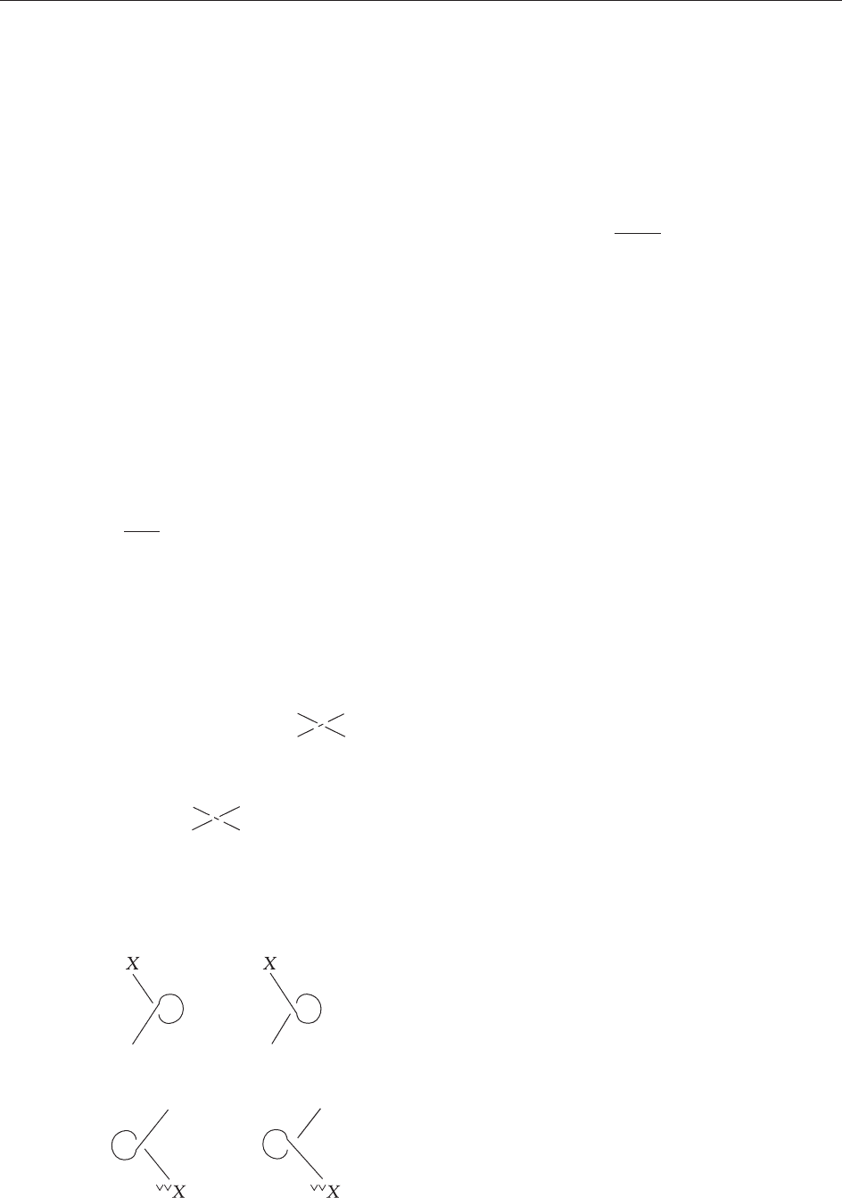
Morphisms constructed from braidings and (co)-

evaluations are often described by tangles. The

conventions are listed in Figure 1. The suggested

assignment of morphisms in C to elementary pictures

extends to a unique functor  from the category of

C-colored tangles to the category C itself. With the

above interpretation, these tangles need not be

oriented. We shall use the same notation for framed

tangles, and the framing will be within the plane.

The maps Ob C!Ob C, X 7!X

,andX 7!

extend to contravariant self-equivalences C!C,

f 7!f

, and f 7!

f . For given f, the morphisms f

and

f can be defined, respectively, by the following

pictures using the assignment from Figure 1:

∨

We have a monoidal self-equivalence of C,

ð

Þ: ðC;; 1Þ!ðC; ;1Þ; X7!X

; f 7!f

2X;Y

¼ X

Y

jþ

ðY

X

!

1t

ðX YÞ



½1

It is not always true that the two duals X

and

are isomorphic. However, there are canonical

isomorphisms

X !

ðX

Þ; X !ð

XÞ

A morphism

f :

X Y by

X,Y

X Y Y X

The braiding

–1

X Y Y X

The inverse braiding

X X

∨

The evaluation

∨

coev

∨

The coevaluation

Figure 1 Conventions for notation of morphisms from

tangles.

Braided and Modular Tensor Categories 353

We may replace the category C with an equivalent one,

such that the above isomorphisms become identity

morphisms, and the functors 

and

 are inverse to

each other. We shall assume this to simplify notations.

Finally, we denote the iterated duals by X

(n_)

= X

__

(n times) and X

(n_)

__

X (n times) for n  0.

Braided Categories

Here we review the definitions of the braiding

isomorphism and further derived isomorphisms. Sev-

eral basic relations between them are listed. Two

important classes of examples of braided categories

are given by the categories of modules over quasitrian-

gular Hopf algebras and the categories of tangles.

Definition 4 A braided category (C, c) is a monoidal

category C equipped with a functorial isomorphism

c = c

X, Y

: X  Y !Y  X – the braiding, or the

commutativity isomorphism – such that the two

hexagons commute,

X ðY  ZÞ

1c

1

X ðZ  YÞ!

ðX  ZÞY

a ##c

1

 1

ðX  YÞZ !

1

Z ðX  YÞ!

ðZ  XÞY

(one for c and one for c

1

The graphical notation for the braiding and its

inverse is

c ¼ðc

X;Y

: X  Y ! Y  X Þ¼

c ¼

In a rigid braided category, we can define

functorial isomorphisms using again the conventions

from Figure 1:

∨∨

–1

–2

–1

–2

–1

These are isomorphisms of monoidal functors

(see [1])

: ðId; c

2

Þ!ð

; j

1

: ðId; c

Þ!ð

; j

In particular, this implies the commutativity of the

diagram

X  Y

2

X  Y

u

##u

 Y

!

ðX  YÞ

The square of the monoidal functor (

, j

)is

ð

____

; j

Þ : ðC; ; 1Þ!ðC; ; 1Þ;

X 7!X

____

; f 7!f

tttt

where

4X;Y

¼ X

____

Y

____

!

ðX

Y

!

ðX YÞ

____



The natural isomorphism u

= u

1

 u

is, in fact, an

isomorphism of monoidal functors u

: (Id, id) !

(

____

, j

Ribbon Categories

Now we define balancing and recall some properties

of balanced (ribbon) categories.

Definition 5 Let C be a rigid braided category.

Abalancing

: X !X

is an isomorphism of

monoidal functors  : (Id, id, id) !(

, j

, d

)such

that 

= u

and 

= 

1

: X

___

.Thecate-

gory C equipped with a balancing is called

balanced.

We also use the notation u

= . In any balanced

category, there exists a canonical ribbon twist v.

A ribbon twist v = v

: X !X, v :Id!Id is a self-

adjoint (v

= v

) automorphism of the identity

functor such that c

= (v

1

 v

1

)  v

XY

. It can be

determined from the equations

¼ u

 v

1

¼ u

1

 v : X ! X



1

¼ u

2

¼ u

2

 v

1

¼u

2

1

 v : X !

In particular, its square is given by the canonical

isomorphism v

= u

2

 u

. Conversely, in any

rigid braided category with a ribbon twist (called

ribbon category) there exists a canonical balan-

cing u

given b y the above for mulas. Thus, ribbon

categories and balanced categories are synonyms.

In the case of X = 1,wehavev

= id

354 Braided and Modular Tensor Categories