Francoise J.-P., Naber G.L., Tsun T.S. (editors) Encyclopedia of Mathematical Physics

Подождите немного. Документ загружается.

to be fundamental when computer speeds approach

saturation. Moreove r, CAs themselves can mimic

parallel computations, see, for example, Figure 19,

where a nonlocal CA ‘‘computes’’ very efficiently the

celebrated Collatz–Ulam 3n þ 1 map.

CAs in Physics

Since Newton, physics has been described through

differential equations and continuous functions.

However, such a mathematical description is not

fit for simulation on a computer, and some

discretizations must be considered. First, one has to

discretize space and time passing from differential

equations to (finite systems of) finite difference

equations; second, one has to round off the values

of the functions to store them in the memory of the

computer. The main drawback of this procedure is

that in chaotic systems such approximations can

rapidly lead to great differences between the real

and the simulated behavior. As already noticed, this

problem does not appear in CA. Thus, one would

like to use this good characteristic of CAs in physical

modeling takin g due accoun t of the continuous

nature of the physics involved. This requires atten-

tion and ingenuity in constructing reliable CA

models for physical processes. For example, this

goal has been achieved in the so-called lattice gas

automata (LGAs).

LGAs are CA models for the microscopic

dynamics of fluids and gases. The thermodynamic

limit of these CAs yields the correct continuous

functions for the macroscopic quantities (density,

pressure, viscosity, etc.).

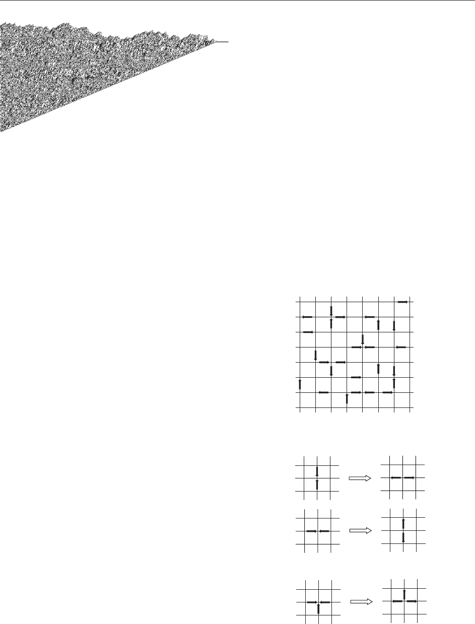
The first step toward LGAs was the disco very that

the HPP model developed in the 1970s by Hardy,

Pomeau and De Pazzis was in fact a CA. The HPP

model describes the behavior of a fluid (or a gas) in

a plane. The configuration space is given by a

bidimensional square lattice and the particles are

described by arrows lying on the edges of the lattices

and pointing to some vertex (see Figure 20a).

The particles are assumed to be all identical and

with the same velocity, an d particles on the same

edge with the same direction are not allowed

(exclusion principle). The EL prescribes that parti-

cles move with unitary velocity along the edges in

the direction pointed by the arrow (free flight)

unless there are exactly two particles on the edges

connected to a given vertex and they point in

opposite directions (collision); in this case they are

replaced by two arrows pointing outward on the

previously empty edges (see Figure 20b). Clearly,

the EL conserves the number and the momentum of

the particles.

The HPP model can be described algebraically.

The admissible particle velocities are just

¼þ

x; c

¼þ

y; c

¼

x; c

¼

y ½26

Figure 19 A CA that ‘‘computes’’ the 3n þ 1 Collatz–Ulam

map. The ID for the CA is the initial number for the iterated map

(binary notation, order 2

300

, randomly chosen, displayed on the

left vertical axis). The CA, according to the Collatz conjecture,

ends up to the final stable configuration (horizontal line on the

right for the CA, 1 !4 !2 !1 for the map).

(a)

(b)

Collisions

Free flight

Figure 20 (a) An example of configuration for the HPP model.

(b) Head on collisions and three particle collisions in the HPP

model.

Cellular Automata 465

Accordingly, only four bits n

(x, t), j = 1, 2, 3, 4, are

required to denote the presence (1) or the absence

(0) of a particle with velocity c

pointing vertex x at

time t. The dynamical rule for HPP can be written in

the form

ðx þ c

; t þ 1Þ¼n

ðx; tÞþ!

ðx; tÞ½27

where term n

(x, t) on the right-hand side accounts

for the free flight of particles, while !

(x, t) modifies

the trajectories in the case of collisions. The !

are

determined by the state of the system according to

the following rules:

¼n

ð1  n

Þn

ð1  n

þð1  n

Þn

ð1  n

Þn

½28a

¼n

ð1  n

Þn

ð1  n

þð1  n

Þn

ð1  n

Þn

½28b

¼n

ð1  n

Þn

ð1  n

þð1  n

Þn

ð1  n

Þn

½28c

¼n

ð1  n

Þn

ð1  n

þð1  n

Þn

ð1  n

Þn

½28d

It is plain that eqns [27] and [28] can be

interpreted as the EL for a CA.

In the thermodynamic limit, the equations govern-

ing the dynamics of the macroscopic quantities of

the fluid are given by the continuity equation and by

anisotropic Navier–Stokes equations. The aniso-

tropy in the Navier–Stokes equations is due to the

fact that the invariance group of the square lattice is

too small. This problem was solved by Frisch,

Hasslacher, and Pomeau in 1986, with the introduc-

tion of the FPP model. It turns out that a hexagonal

lattice has enough symmetries to recover the

isotropic Navier–Stokes equations in the thermo-

dynamic limit. So, the FPP model is an example of a

model where even if the microscopic dynamics is

almost a caricature of the real dynamics, the

thermodynamic limit gives rise to the correct

physical equations.

CAs have been used to simulate many other

physical processes (unfortunately, there is no space

here for a sufficiently elaborate description). The

principal fields of application are: percolation

theory, magneti sm, diffusion phenomena, sandpiles,

models of earthquakes, crystal growth, etc.

The more intriguing aspect of some even simple CAs

(e.g., CA9, CA10: see Figures 16 and 18) is their very

rich particle-like dynamics. For instance, the existence

of solitonic collisions suggested that the techniques

recently developed to find and treat ‘‘integrable’’

nonlinear dynamical systems (nonlinear continuous

and discrete evolution equations, many-body pro-

blems) could profitably be extended to find ‘‘integr-

able’’ CAs. Indeed, many such CAs have been found

that exhibit ‘‘solitons’’ and are endowed with non-

trivial conservation laws (of course, this is very

important in physical modeling). Moreover, the

above-cited similarity between certain CA behaviors

and elementary particle physics phenomena suggests

that the fundamental structure of reality (at the Planck

level) could indeed be that of a CA (cells of Plank

length, discrete time flow): attempts to construct this

underlying CA physics have been pursued.

Other Applications

CAs exhibit a great plasticity, which makes them

well suited to model systems in a wide range of

fields. This is mainly due to the fact that CAs with

very simple rules can also simulate universal Turing

machines, so that they can exhibit a very rich and

complicated overall dynamics (in principle, one

could simulate any dynamical system using a simple

CA). There is another reason for the wide applic-

ability of CA modeling even outside of physics:

namely, it is well known that algorithms, not

differential equations, are better instruments to

schematize dynamical processes for complex and

organized systems . Since simple algorithms can be

naturally implemented on CAs, the latter are very

useful for realizing simple models and simulations in

many fields: biology, economics, ecology, neural

networks, traffic models, etc.

Moreover, applications of CAs in informatics and

specifically in cryptography and data compression

have been investigated.

See also: Dynamical Systems in Mathematical Physics:

An Illustration from Water Waves; Generic Properties of

Dynamical Systems; Integrable Systems: Overview.

Further Reading

Berlekamp ER, Conway JH, and Guy R (1982) Winning Ways for

Your Mathematical Plays. London: Academic Press.

Boghosian BM (1999) Lattice gases and cellular automata. Future

Generation Computer Systems 16: 171–185.

Boon JP, Dab D, Kapral R, and Lawniczak A (1996) Lattice gas

automata for reactive systems. Physics Reports 273: 55–147.

Burks AW (ed.) (1970) Essay on Cellular Automata. Urbana:

University of Illinois Press.

Chopard B and Droz M (1998) Cellular Automata Modeling of

Physical Systems. Cambridge: Cambridge University Press.

Doolen G (ed.) (1990) Lattice Gas Methods for Partial

Differential Equations. New York: Addison-Wesley.

Gardner M (1983) Wheels, Life, and Other Mathematical

Amusements. New York: W H Freeman.

466 Cellular Automata

Jackson EA (1990) Perspectives of Nonlinear Dynamics.

Cambridge: Cambridge University Press.

Toffoli T and Margolus N (1987) Cellular Automata Machines –

A New Enviroment for Modeling. Cambridge: The MIT Press.

von Neumann J (1966) In: Burks AW (ed.) Theory of Self-

Reproducing Automata. Urbana: University of Illinois Press.

Wolfram S (2002) A New Kind of Science. Champaign: Wolfram

Media.

Central Manifolds, Normal Forms

P Bonckaert, Universiteit Hasselt, Diepenbeek,

Belgium

Introduction

We consider differentiable dynamical systems gen-

erated by a diffeomorphism or a vector field on a

manifold. We restrict to the finite-dimensional case,

although some of the ideas can also be developed in

the general case (Vanderbauwhede and Iooss 1992).

We also restrict to the behavior near a stationary

point or a periodic orbit of a flow.

Let the origin 0 of R

be a stationary point of a C

vector field X, that is, X(0) = 0. We consider the

linear approxim ation A = dX(0) of X at 0 and its

spectrum (A), which we decompose as (A) = 

[



[ 

, where 

resp. 

consists of those

eigenvalues with real part <0 resp. = 0 resp. >0. If



= ; then there is no central manifold, and the

stationary point 0 is called hyperbolic. Let E

, E

and E

be the linear A-invariant subspaces corre-

sponding to 

resp. 

. Then R

= E



 E

. We look for corresponding X-invariant

manifolds in the neighborhood of 0, in the form of

graphs of maps. More precisely:

Theorem 1 Let the vector field X above be of class

(1 r < 1). There exist map germs 

:(E

,0)!

E

, 

:(E

E

,0)!E

, 

:(E

,0)! E

E



:(E

E

,0)!E

, and 

:(E

,0)!E

E

class C

such that the graphs of these maps are

invariant for the flow of X. Moreover, these maps

are of class C

, and their linear approximation at 0

is zero, that is, their graphs are tangent to,

respectively, E

E

, E

E

, and E

. If X is

of class C

then 

and 

are also of class C

. If

X is analytic then 

and 

are also analytic.

The graph of 

is called the (local) central

(or, center) manifold of X at 0 and it is often

denoted by W

. Thus, it is an invariant manifold

of X tangent at the generalized eigenspace of

dX(0) corresponding to the eigenvalues having zero

real part.

(Non) uniqueness, Smoothness

Most proofs i n the literature (Vanderbauwhede

1989) use a cutoff in order to construct globally

defined objects, and then obtain the invariant graph

as the solution of s ome fixed-point problem of a

contraction in an appropriate function space.

Although this solution is unique for the globalized

problem, this is not the case at the germ level:

another cutoff may produce a different germ of

a central manifold. In other words, locally a

central manifold might not be unique, as is

easily seen on the planar e xample x

@=@x 

y@=@y. On the other hand, the 1-je t of the map



,incaseofaC

vector field, is unique, so if

there would exist an analyti c central manifold then

this last one is unique; in the foregoing example,

it is the x-axis. But for the (polynomial) example

(x  y

)@=@x þ y

@=@y one can calculate that the

1-jet of x = 

(y)isgivenbyj



(y) =

n1

n!y

nþ1

which has a vanishing radius of convergence, so

there is no analytic central manifold. On t he other

hand, by the Borel theorem we c an choose a

-representative for 

. This can be generalized

in the planar case:

Proposition 1 If n = 2 and if X is C

and if the

1-jet of X in the direction of the central manifold

is nonzero, then this central manifold is C

In particular, if X is analytic then the central

manifold is either an analytic curve of stationary

points or is a C

curve along which X has a

nonzero jet.

For proofs and additional reading, the reader is

referred to Aulbach (1992). In general, a central

manifold is not necessarily C

(van Strien 1979,

Arrowsmith and Place 1990): for the system in

given by

ðx

 z

þðy þ x

 z

þ 0 

one can find a C

central manifold for every k but

there is no C

central manifold. Indeed, in this case

the domain of definition of 

shrinks to zero when

k tends to infinity.

Central Manifolds, Normal Forms 467

Central Manifold Reduction

The importance of a central manifold lies in the

principle of central manifold reduction, which

roughly says that for local bifurcation phenomena

it is enough to study the behavior on the central

manifold, that is, if two vector fields, restricted to

their central manifolds, have homeomorphic integral

curve portraits, and if the dimensions of E

and E

are equal, then the two vector fields have home-

omorphic integral curve portraits in R

, at least

locally near 0. Let us be more precise:

Theorem 2 Let m be the dimension of E

. There

exists p,0 p  n  m, such that X is locally

-conjugate to

i¼1

ðz

; ...; z

mþp

i¼mþ1



i¼mþpþ1

where (z

, ..., z

) is a coordinate system on a

central manifold,(z

, ..., z

) is a coordinate system

on R

extending (z

, ..., z

) and

i = 1

@=@z

is the restriction of X to a central manifold.

Moreover, if

Y ¼

i¼1

ðz

; ...; z

mþp

i¼mþ1



i¼mþpþ1

and if

i = 1

@=@z

is C

-equivalent (resp. C

conjugate) to

i = 1

@=@z

then X is C

-equivalent

(resp. -conjugate) to Y.

For a proof and further reading (a generalization)

see Palis and Takens (1977).

In case that more smoothness than just C

needed, we have the principle of normal lineariza-

tion along the central manifold. More concretely, let

x denote a coordinate in the central manifold and

let y be a complementary variable, that is, let

X = X

@=@x þ X

@=@y. We define the normally

linear part along the central manifold by

NX :¼ X

ðx; 0 Þ

ðx; 0Þy

Under certain nonresonance conditions (Takens

1971, Bonckaert 1997) on the real parts of the

eigenvalues of dX(0), there exists a C

local

conjugacy between X and NX for each r 2 N

(assuming X to be of class C

). If there are

resonances, then one can conjugate with the

so-called seminormal or renormal form containing

higher-order terms (see Bonckaert (1997 , 2000) and

references therein; here one can also find results for

cases where extra constraints should be respected,

like symmetry, reversibility, or invariance of some

given foliation etc.).

Parameters

Having an eigenvalue with zero real part is

ungeneric, so in bifurcation problems we consider

p-parameter families X



near, say,  = 0. With

respect to the results above, we remark that such a

family can be considered as a vector field near

(0, 0) 2 R

 R

tangent to the leaves R

 {}. In

fact, the parameter direction R

is contained in E

In all the results mentioned, this structure ‘‘of being

a family’’ is respected. For example, in Theorem 2

we replace

, ..., z

)by

, ..., z

, ). Hence,



is a versal unfolding of

then X



is a versal

unfolding of X

. By this, the search for versal

unfoldings is reduced to the unfolding of singula-

rities whose linear approximation at 0 has a purely

imaginary spectrum.

Diffeomorphisms, Periodic Orbits

A completely analogous theory can be developed for

fixed points of diffeomorphisms f :(R

,0)! R

Here we split up the spectru m of the linear part

L = df (0) at 0 as (L) = 

[ 

, where 

resp.



resp. 

consists of those eigenvalues with

modulus <1 resp. = 1 resp. >1. This theory can be

applied to the time-t map of a vector field (and will

give the same invariant manifolds) and to the

Poincare´ map of a transversal section of a period ic

orbit of a vector field (Chow et al. 1994).

Normal Forms

The general idea of a normal form is to put a

(complicated) system into a form ‘‘as simple as

possible’’ by means of a change of coordinates. This

idea was already developed to a great extent by

H Poincare´. Simple examples are: (1) putting a square

matrix into Jordan form, (2) the flow box theorem

(Arrowsmith and Place 1990) near a nonsingular

point. Depending on the context and on the purpose

of the simplification, this concept may vary greatly. It

depends on the kind of changes of coordinates that are

tolerated (linear, polynomial, formal series, smooth,

analytic) and on the possible structures that must be

preserved (e.g., symplectic, volume-preserving, sym-

metric, reversible etc.). Let us restrict to local normal

forms, that is, in the vicinity of a stationary point of a

vector field or a diffeomorphism (the latter can be

468 Central Manifolds, Normal Forms

applied to the Poincare´ map of a periodic orbit). We

concentrate on the simplification of the Taylor series.

The general idea is to apply consecutive polynomial

changes of variables; at each step we simplify terms of

a degree higher than in the step before. The ideal

simplification would be to put all higher-order terms

to zero, which would (at least at the level of formal

series) linearize the system. But as soon as there are

resonances (see below), this is impossible: the planar

system 2x@=@x þ (y þ x

)@=@y cannot be formally

linearized.

Setting

Let X be a C

rþ1

vector field defined on a neighbor-

hood of 0 2 R

, and denote A = dX(0) (its linear

approximation at 0). The Taylor expansion of X at

0 takes the form

XðxÞ¼A  x þ

k¼2

ðxÞþOðjxj

rþ1

where X

2 H

, the space of vector fields whose

components are homogeneous polynomials of

degree k. The classical formal normal-form theorem

is as follows. We define the operator L

on H

putting L

h(x) = dh(x)  A  x  A  h(x); one calls L

the homological operator. One checks that

)  H

. One also denotes this by ad A(h)(x):

see further in the Lie algebra setting. Let R

be the

range of L

, that is, R

= L

). Let G

denote any

complementary subspace to R

in H

. The formal

normal-form theorem states, under the above

settings:

Theorem 3 (Chow et al. 1994, Dumortier 1991)

There exists a composition of near identity changes

of variables of the form

x ¼ y þ 

ðyÞ½1

where the components of 

are homogeneous

polynomials of degree k, such that the vector field

X is transformed into

YðyÞ¼A  y þ

k¼2

ðyÞþOðjyj

rþ1

where g

2 G

, k = 2, ..., r.

Sometimes this theorem is applied to the restric-

tion of a vector field to its central manifold, for

reasons explained in the last section. This is the

reason why we did not assume X to be C

;inthe

latter case one can let r !1and obtain a normal

form on the level of formal Taylor seri es (also called

1-jets). Using a theorem of Borel, we infer the

existence of a C

change of variables  such that

the Taylor series of 



(X)isA  y þ

k = 2

(y). For

practical computations, it is often appropriate to

first simplify the linear part A and to diagonalize it

whenever possible. Hence, it is convenient to use a

complexified setting and to use complex polyno-

mials or power series. One can show that all

involved changes of variables preserve the property

of ‘‘being a complex system coming from a real

system,’’ that is, at the final stage we can return to a

real system (see, e.g., Arrowsmith and Place (1990)

for a more precise mathematical description).

Hence, we can assume that A is an upper

triangular matrix. Let the eigenvalues be 

, ..., 

It can be calculated that the eigenvalues of L

,asan

operator H

! H

, are then the num bers h, i

where  2 N

j = 1



= k and 1  j  n. Hence, if

these would all be nonzero then B

= H

, and then

we have an ideal simplification, that is, all g

equal

to zero. However, if such a number is zero, that is,

h; i

¼ 0 ½2

it is called a resonance between the eigenvalues. In

such a case, we have to choose a complementary

space G

. From linear algebra it follows that one

can always choose

¼ kerðL



Þ½3

where A



is the adjoint operator. But this choice [3] is

not unique and is, from the computational point of

view, not always optimal, especially if there are

nilpotent blocks. This fact has been exploited by

many authors. A typical example is the case where

A = y@=@x. On the other hand, if A is semisimple we

can choose the complementary space to be ker(L

), so

= 0; we can assume it to be the (complex)

diagonal[

, ..., 

]. In that case we can be more

explicit as follows. Let e

= @=@x

denote the standard

basis on C

. For a monomial one can calculate that

ðx



Þ¼ðh; i

Þx



½4

If the latter is zero, then the monomial is called

resonant. This implies that the normal form can be

chosen so that it only contains resonant mon omials.

Putting a system into normal form not only

simplifies the original system, it also gives more

geometric insight on the Taylor series. To be more

precise, suppose (for simplicity, this can be genera l-

ized (Dumortier 1997)) that A is semisimple. One

can calculate that the condition L

= 0 implies:

exp (At)g

( exp (At)x) = g

(x) for all t 2 R. This

means that g

is invariant for the one-parameter

group exp(At). A typical example in the plane

is: A has eigenvalues i, i. Note that the (only)

resonances are h(i , i), (p þ 1, p)ii = 0 and

Central Manifolds, Normal Forms 469

h(i, i), (p, p þ 1)iþi = 0 for all p 2 N.We

suppose that the original system was real, that is,

on R

; we can choose linear coordinates such that

for z = x þ iy,



z = x  iy the linear part is

A = diagonal[i, i ]. Applying the remarks above,

we conclu de that the normal form only contains the

monomials (z



z@=@z and (z



z@=@



z. The geo-

metric interpretation here is that these monomials

are invariant for rotat ions around (0, 0). This can

also be seen on the real variant of this: the Taylor

series of the (real) normalized system has the

form ( þ f (x

þ y

))(x@=@y  y@=@x) þ g(x

þ y

)

(x@=@x þ y@=@y) and is invariant for rotations.

Warning: the dynamic behavior of a formal normal

form in the central manifold can be very different

from that of the original vector field, since we are

only looking at the formal level. A trivial example is

(take f = g = 0 in the foregoing example) X(x, y) =

(x@y  y@x)  exp (1=(x

))@=@x, where orbits

near (0, 0) spiral to (0, 0), whereas the normal form

is just a linear rotation. This difference is due to the

so-called flat terms, that is, the difference between

the transformed vector field and a C

-realization of

its normalized Taylor series (or polynomial). In case

of analyticity of X, one can ask for analyticity of the

normalizing transformation . Generically, this is

not the case in many situations. The precise meaning

of this ‘‘genericity condition’’ is too elaborate to

explain in this brief review article. We provide some

suggestions for further reading in the next section.

One could roughly say that, in the central manifold,

the normal form has too much symmetry and is too

poor to model more complicated dynamics of the

system, which can be ‘‘hidden in the flat terms.’’ To

quote Il’yashenko (1981): ‘‘In the theory of normal

forms of analytic differential equations, divergence

is the rule and convergence the exception ....’’

In many applications, we want to preserve some

extra structure, such as a symplectic structure, a

volume form, some symmetry, reversibility, some

projection etc.; the case of a projection is important

since it includes vector fields depending on a para-

meter. Sometimes a superposition of these structures

appears (e.g., a family of volume-preserving systems).

We would like that the normal-form procedure

respects this structure at each step. One can often

formulate this in terms of vector fields belonging to

some Lie subalgebra L

. The idea is then to use

changes of variables like [1], where 

is then generated

by a vector field in L

. This will guarantee that all

changes of variables are ‘‘compatible’’ with the extra

structure. Unlike the general case where we could

work with monomials as in [4], we will have to

consider vector fields h

in L

whose components are

homogeneous polynomials of degree k.Ifthiscanbe

done, one says that L

respects the grading by the

homogeneous polynomials. In order to fix ideas,

suppose that L

are the divergence-free planar vector

fields. Note that a monomial x

@=@x is not diver-

gence free. We can instead use time mappings of

homogeneous vector fields of the form a(q þ

1)x

pþ1

@=@x  a( p þ 1) x

qþ1

@=@y.Uptoterms

of higher order we can use the time-one map of h

instead of x þ h

(x). In case that one asks for a C

realization of the normalizing transformation, we need

an extra assumption on the extra structure, that is, on

, called the Borel property: denote by J

1,0

the set of

formal series such that each truncation is the Taylor

polynomial of an element of L

. The extra assumption

is: each element of J

1,0

must be the Taylor series of a

vector field in L

. It can be proved (Broer 1981)

that the following structures respect the grading and

satisfy the Borel property: being an r-parameter family,

respecting a volume form on R

, being a Hamiltonian

vector field (n even), and being reversible for a linear

involution.

One could consider other types of grading of the

Lie-algebras involved.

This method, using the framework of the so-called

filtered Lie algebras, is explained and developed

systematically in a more general and abstract

context in Broer (1981).

In nonlocal bifurcations, such as near a homo-

clinic loop, for example, it is not enough to perform

central manifold reduction near the singularity: a

simplified smooth model in a full neighborhood of

the singularity is often needed, for example, in order

to compute Poincare´ maps.

Let us start with the ‘‘purely’’ hyperbolic case (i.e.,

dim E

= 0). First we compute the formal normal

form such as the above. If there are no resonances

[2] then we can formally linearize the vector field X.

If X is C

then a classical theorem of Sternberg

(1958) states that this linearization can be realized

by a C

change of variables (i.e., no more flat terms

remaining). In case there are resonances, we must

allow nonlinear terms: the resonant monomials. In

this case we can also reduce C

to this normal form.

Using the same methods, it is also possible to reduce

to a polynomial normal form, but this time using

(k < 1) changes of variables. More precisely, if k

is a given number and if we write the vector field as

X = X

þ R

, where X

is the Taylor polynomial

up to order N (which can be assumed to be in

normal form) and where R

(x) = O(jxj

Nþ1

), then for

N sufficiently large there is a C

change of variables

conjugating X to X

near 0. The number N depends

on the spectrum of A = dX(0). An elegant proof of

these facts can be found in Il’yashenko and Yakovenko

(1991). For the case when extra structure must be

470 Central Manifolds, Normal Forms

preserved, see Bonckaert (1997), which also deals with

the partially hyperbolic case (dim E

 1). As already

remarked above, the case of a parameter-dependent

family can be regarded as a partially hyperbolic

stationary point preserving this extra structure.

The question of an analytic normal form, also in

the hyperbolic case, leads to convergence questions

and calls upon the so-called small-divisor problems.

The classical results are due to Poincare´ and Siegel.

Let us summarize them; they are formulated in the

complex analytic setting:

Theorem 4

(i) If the convex hull of the spectrum of A does not

contain 0 2 C then X can locally be put into

normal form by an analytic change of variables.

Moreover, this normal form is polynomial.

(ii) If the spectrum {

, ..., 

} of A satisfies the

condition that there exists C > 0 and >0 such

that for any m 2 N

with

 2:

jhð

; ...;

Þ; mi

j

jmj



½5

for 1  j  n then X can be locally linearized by

an analytic change of variables.

Note that case (i) contains the case where 0 is a

hyperbolic source or sink. This case (i) in Theorem 4

can be extended if there are parameters: if X

depends analytically on a parameter " 2 C

near

" = 0 then the change of variables is also analytic in

"; moreover, the normal form is then a polynomial

in the space variables whose coefficients are analy-

tically dependent on the parameter " .

For case (ii) this is surely not the case, since the

condition [5] is fragile: a small distortion of the

parameter generically causes resonanc es, be it of a

high order. To fix ideas, consider n = 2 and suppose



< 0 <

. By a generic but arbitrary small

perturbation, we can have that the ratio of these

eigenvalues becomes a negative rational number

p=q, which gives a resonance of the form [2]

with j = 1 and  = (q þ 1, p), so [5] is violated.

So analytic linearization, or even a polynomial

analytic normal form, is ungeneric for families of

such hyperbolic stationary points. The search for

analytic normal forms, that is, simplified models, for

families is still under investigation. A first simplifica-

tion is obtained via the stable and unstable manifold

from Theorem 1, that is, the graphs of 

and 

When X is analytic near 0 then these manifolds are

also analytic. So, up to an analytic change of variables,

we can assume that E

and E

are invariant, which

gives a simplification of the expression of X.More-

over, there is analytic dependence on parameters.

For local diffeomorphisms there are completely

similar theorems pertaining to all the cases consid-

ered above.

Concluding Remarks

The concept of central manifold can be extended to

more general invariant sets (see Chow et al. (2000)

and references therein). It can also be extended to

the infinite-dimensional case and can be applied to

partial differential equations (Vanderbauwhede and

Iooss 1992).

Concerning the generic divergence of normalizing

transformations, the reader is referred to Broer and

Takens (1989), Bruno (1989), Il’yashenko (1981),and

Il’yashenko and Pyartli (1991). Although the power

series giving the normalizing transformation generally

diverges, the study of the dynamics is often performed

by truncating the normal form at a certain order.

Recently, Iooss and Lombardi (2005) considered the

question as to what an optimal truncation is. It is

shown, in case dX(0) is semisimple, that the order of

the normal form can be optimized so that the remainder

satisfies some estimate shrinking exponentially fast to

zero as a function of the radius of the domain.

Concerning normal forms preserving the

Hamiltonian structure, see Birkhoff (1966) and

Siegel and Moser (1995) for a starting point; this is

an extended subject on its own, sometimes called

Birkhoff normal form, and it would require another

review article.

Further simplifications of the normal form can

sometimes be obtained by taking into account

nonlinear terms (instead of just A) in order to obtain

reductions of higher-order terms (see Gaeta (2002)

and especially the references therein).

Applications of normal forms and central mani-

folds to bifurcation theory have been explained in

Dumortier (1991).

See also: Averaging Methods; Bifurcation Theory;

Dynamical Systems and Thermodynamics; Dynamical

Systems in Mathematical Physics: An Illustration from

Water Waves; Finite Group Symmetry Breaking;

Korteweg–de Vries Equation and Other Modulation

Equations; Multiscale Approaches; Normal Forms and

Semiclassical Approximation; Symmetry and Symmetry

Breaking in Dynamical Systems.

Further Reading

Arrowsmith D and Place C (1990) Dynamical Systems. Cambridge:

Cambridge University Press.

Aulbach B (1992) One-dimensional center manifolds are C

Results in Mathematics 21: 3–11.

Central Manifolds, Normal Forms 471

Birkhoff GD (1966) Dynamical Systems. With an addendum by

Jurgen Moser. American Mathematical Society Colloquium

Publications, vol. IX. Providence, RI: American Mathematical

Society.

Bonckaert P (1997) Conjugacy of vector fields respecting

additional properties. Journal of Dynamical and Control

Systems 3: 419–432.

Bonckaert P (2000) Symmetric and reversible families of vector

fields near a partially hyperbolic singularity. Ergodic Theory

and Dynamical Systems 20: 1627–1638.

Broer H (1981) Formal normal forms for vector fields and some

consequences for bifurcations in the volume preserving case.

In: Dynamical Systems and Turbulence, Warwick 1980,

vol. 898, Lecture Notes in Mathematics. New York: Springer.

Broer H and Takens F (1989) Formally symmetric normal forms

and genericity. Dynamics Reported. A Series in Dynamical

Systems and their Applications 2: 11–18.

Bruno AD (1989) Local Methods in Nonlinear Differential

Equations. New York: Springer.

Chow S-N, Li C, and Wang D (1994) Normal Forms and

Bifurcations of Planar Vector Fields. Cambridge: Cambridge

University Press.

Chow S-N, Liu W, and Yi Y (2000) Center manifolds for invariant

sets. Journal of Differential Equations 168: 355–385.

Dumortier F (1991) Local study of planar vector fields: singula-

rities and their unfoldings. In: Van Groesen E and De Jager EM

(eds.) Structures in Dynamics, Studies in Mathematical Physics,

vol. 2, pp. 161–241. Amsterdam: Elsevier.

Gaeta G (2002) Poincare´ normal and renormalized forms. Acta

Applicandae Mathematicae 70(1–3): 113–131 (symmetry and

perturbation theory).

Il’yashenko YS (1981) In the theory of normal forms of analytic

differential equations violating the conditions of Bryuno

divergence is the rule and convergence the exception. Moscow

University Mathematical Bulletin 36(2): 11–18.

Il’yashenko YS and Pyartli AS (1986) Materialization of reso-

nances and divergence of normalizing series for polynomial

differential equations. Journal of Mathematical Sciences

32(3): 300–313.

Il’yashenko YS and Yakovenko SY (1991) Finitely smooth normal

forms of local families of diffeomorphisms and vector fields.

Russian Mathematical Surveys 46: 1–43.

Iooss G and Lombardi E (2005) Polynomial normal forms with

exponentially small remainder for analytic vector fields.

Journal of Differential Equations 212: 1–61.

Palis J and Takens F (1977) Topological equivalence of normally

hyperbolic dynamical systems. Topology 16(4): 335–345.

Siegel CL and Moser JK (1971) Lectures on Celestial Mechanics,

(reprint 1995). Berlin: Springer.

Sternberg S (1958) On the structure of local homeomorphisms of

Euclidean n-space. II. American Journal of Mathematics

80: 623–631.

Takens F (1971) Partially hyperbolic fixed points. Topology

10: 133–147.

Vanderbauwhede A (1989) Center manifolds, normal forms and

elementary bifurcations. In: Kirchgraber U and Walther O

(eds.) Dynamics Reported, vol. 2, pp. 89–169. New York:

Wiley.

Vanderbauwhede A and Iooss G (1992) Center manifold theory in

infinite dimensions. In: Jones CKRT et al. (eds.) Dynamics

Reported, vol. 1, New Series, pp. 125–163. Berlin: Springer.

Channels in Quantum Information Theory

M Keyl, Universita

di Pavia, Pavia, Italy

Introduction

Consider a typical quantum system such as a string

of ions in a trap. To ‘‘process’’ the quantum

information the ions carry, we have to perform in

general many steps of a quite different nature.

Typical examples are: free time evolution (including

unwanted but unavoidable interactions with the

environment), controlled time evolution (e.g., the

application of a ‘‘quantum gate’’ in a quantum

computer), preparations and measurements. Each

processing step can be described by a channel which

transforms input systems into output system of a

possibly different type (e.g., a measurement trans-

forms quantum systems into classi cal information).

Systems, States, and Algebras

To get a unified mathematical description of systems

of different physical nature, it is useful to consider



-algebras (which are, in our case, always finite

dimensional): quantum systems can be represented

in terms of the algebra B(H) of (bounded) operators

on the Hilbert space H= C

; for classical informa-

tion we have to choose the set C(X) of (continuous),

complex-valued functions on the finite alphabet X;

and the tensor product of both B(H) C( X)

describes hybrid systems which are half-classical

and half-quantum. Assume now that A is one of

these algebras. Effects (i.e., yes/no measurements on

the system in question) are then described by A 2A

satisfying 0  A  1, stat es are positive, normalized

linear functionals ! : A!C, and the probability to

get the result ‘‘yes’’ during an A measurement on a

system in the state ! is given by !(A). Since A is

assumed to be finite dimensional, each state ! on

B(H) is represented by a density operator , that is,

!(A) = tr(A). Likewise, a state ! on C(X) has the

form !(A) =

A(x)p

, where ( p

)

x2X

denotes a

probability distribution on X, and a state ! on

B(H) C(X) is described by a sequence (

)

x2X

positive (trace-class) operators on B(H) with

tr(

) = 1 such that !(A) =

tr(

). Here

472 Channels in Quantum Information Theory

we have used the fact that an element A 2B(H) 

C(X) can be represented in a canonical way by a

sequence (A

)

x2X

of operators on H. The set of

states will be denoted in the following by S(A) and

the set of effects by E(A).

Completely Positive Maps

Our aim is now to get a mathematical object which

can be used to describe a channel. To this end,

consider two C



-algebras, A, B, describing the input

and output system, respectively, and an effect A 2B

of the output system. If we invoke first a channel

which transforms A systems into B systems, and

measure A afterwards on the output systems, we end

up with a measurement of an effect T(A) on the

input systems. Hence, we get a map T : E(B) !E(A)

which completely describes the channel (note that

the direction of the mapping arrow is reversed

compared to the natural ordering of processing).

Alternatively, we can look at the states and interpret

a channel as a map T



: S(A) !S(B) which trans-

forms A systems in the state  2S(A) into B systems

in the state T



(). To distinguish between both

maps, we can say that T describes the channel in the

Heisenberg picture and T



in the Schro¨ dinger

picture. On the level of the statistical interpretation,

both points of view should coincide of course, that

is, the probabilities (T



)(A)and(TA) to get the

result ‘‘yes’’ during an A measurement on B systems

in the state T



, respectively a TA measurement on

A systems in the state , should be the same. Since



)(A) is linear in A, we see immediately that T

must be an affine map, that is, T(

þ 

) =



T(A

) þ 

T(A

) for each convex linear combina-

tion 

þ 

of effects in B, and this in turn

implies that T can be extended naturally to a linear

map, which we will identify in the following with

the channel itself, that is, we say that Tisthe

channel.

Let us now change slightly our point of view and

start with a linear operator T : A!B.Tobea

channel, T must map effects to effects, that is, T has

to be positive: T(A)  0 8A  0 and bounded from

above by 1,thatis,T(1)  1. In addition, it is natural

to require that two channels in parallel are again a

channel. More precisely, if two channels T : A

and S : A

are given, we can consider the map

T  S which associates to each A  B 2A

A

the

tensor product T(A)  S(B)2B

B

. It is natural to

assume that T  S is a channel which converts

composite systems of type A

A

into B

B

systems. Hence, S  T should be positive as well.

Definition 1 Consider two observable algebras

A, B and a linear map T : A!BB(H).

(i) T is called positive if T(A)  0 holds for all

positive A 2A.

(ii) T is called completely positive (CP) if T 

Id : AB(C

) !B(H) B(C

) is positive for

all n 2 N. Here Id denotes the identity map

on B(C

(iii) T is called unital if T(1) = 1 holds.

Consider now the map T



: B



which is dual

to T,thatis,T



(A) = (TA) for all  2B



and A 2A.

It is called the Schro¨ dinger-picture representation of

the channel T, since it maps states to states provided T

is unital. (Complete) positivity can be defined in the

Schro¨ dinger picture as in the Heisenberg picture, and

we immediately see that T is (completely) positive iff



is.

It is natural to ask whether the distinction

between positivity and complete positivity is

really necessary, that is, whether there are

positive maps which are not CP. If at least one

of the algebras A or B is classical, the answer is

no: each positive map is CP in this case. If both

algebras are quantum however, complete positiv-

ity is not implied by positivity alone. The most

prominent example for this fact is the transposi-

tion map.

If item (ii) holds only for a fixed n 2 N,

the map T is called n-positive. This is obviously

a weaker condition than complete positivity.

However, n-positivity implies m-positivity for

all m  n,andforA= B(C

) complete positivity

is implied by n-positivity, provided n  d holds.

Let us consider now the question whether a

channel should be unital or not. We have already

mentioned that T(1)  1 must hold since effects

should be mapped to effects. If T(1) is not equal to 1,

we get (T1) = T



(1)< 1 for the probability to

measure the effect 1 on systems in the state T



,

but this is impossible for channels which produce an

output with certainty, because 1 is the effect which

is always true. In other words, if a CP map is not

unital, it describes a channel which sometimes

produces no output at all and T(1) is the effect

which measures whether we have got an output. We

will assume henceforth that channels are unital if

nothing else is explicitly stated.

Quantum Channels

In this section we will discuss some basic properties

of CP maps which transform quantum systems into

quantum systems, in particular the Stinespring

theorem, which constitutes the most important

structural result. For a more detailed presentation,

including generalizations to more general input/

Channels in Quantum Information Theory 473

output algebras the reader should consult the

textbook by Paulsen (2002).

The Stinespring Theorem

Hence consider channels between quantum systems,

i.e., A= B(H

) and B= B(H

). A fairly simple

example (not necessarily unital) is given in terms of

an operator V : H

by B(H

) 3 A 7!VAV



B(H

). A second example is the restriction to a

subsystem, which is given in the Heisenberg picture

by B(H) 3 A 7!A  1

2B(HK). Finally the com-

position S  T = ST of two channels is again a

channel. The following theorem says that each

channel can be represented as a composition of

these two examples [7].

Theorem 2 (Stinespring dilation theorem). Every

completely positive map T : B(H

) !B(H

) has the

form

TðAÞ¼V



ðA  1

ÞV ½1

with an additional Hilbert space K and an operator

V : H

K. Both (i.e., K and V) can be

chosen such that the span of all (A  1)V with A 2

B(H

) and  2H

is dense in H

K. This

particular decomposition is unique (up to unitary

equivalence) and is called the minimal

decomposition.

By introducing a family j

ih

j of one-dimen-

sional projectors with

j

ih

j= 1, we can define

the ‘‘Kraus operators’’ h , V

i= h  

, Vi.

In terms of these, we can rewrite eqn [1] in

the following form (Kraus 1983):

Corollary 3 (Kraus form). Every CP map

T : B(H

) !B(H

) can be written in the form

TðAÞ¼

j¼1



½2

with operators V

: H

To get a third representation of channels, consider

the Stinespring form [1] of T and a vector 2K

such that U(  ) = V() can be extended to a

unitary map U : HK!HK. It is then easy to

see that the dual T



of T can be written as:

Corollary 4 (Ancilla form). Assume that T : B(H) !

B(H) is a channel. Then there is a Hilbert space K, a

pure state 

, and a unitary map U : HK!HK

such that



ðÞ¼tr

Uð  

ÞU



ðÞ½3

holds.

This representation of a channel has a (seemingly)

very nice physical interpretation, because we can

look at eqn [3] as the unitary interaction of the

system with an unobservable environment, which is

initially in the state 

. The problem, however, is

that there is a great arbitrariness in the choice of U

and 

. This is the weakness of the ancilla form

compared to the Stinespring representation.

Finally, let us state a related result. It characterizes

all decompositions of a given completely positive

map into completely positive summands. By analogy

with results for states on abelian algebras (i.e.,

probability measures), we will call it a Radon–

Nikodym theorem (see Arveson (1969) for a proof).

Theorem 5 (Radon–Nikodym theorem). Let

: B(H

) !B(H

), x 2 X be a family of CP

maps and let V : H

K be the Stinespring

operator of



T =

; then there are uniquely

determined positive operators F

in B(K) with

= 1 and

ðAÞ¼V



ðA  F

ÞV ½4

The Jamiołkowski Isomorphism

The subject of this section is a relation between CP

maps and states of bipartite systems, first discovered

by Jamiołkowski (1972), and which is very useful in

translating properties of bipartite systems into

properties of positive maps and vice versa.

The idea is based on the following setup. Alice

and Bob share a bipartite system in a maximally

entangled state

 ¼

ﬃﬃﬃ

¼1



 e



2HH ½5

(where e

, ..., e

denote an orthonormal basis of H).

Alice applies to her subsystem a channel T : B(H) !

B(H

) while Bob does nothing. At the end of the

processing, the overall system ends up in a state

¼ðT  IdÞjihj½6

Mathematically, eqn [6] makes sense if T is only

linear but not necessarily positive or CP (but then

is not positive either). If we denote the space of

all linear maps from B(H) into B(H

)byL, we get a

map

L3T 7!R

2BðKHÞ ½7

which is easily shown to be linear (i.e.,

TþS

= R

þ R

for all ,  2 C and all

T, S 2L). Furthermore, this map is bijective, hence

a linear isomorphism.

474 Channels in Quantum Information Theory