Griffiths D.F., Higham D.J. Numerical Methods for Ordinary Differential Equations: Initial Value Problems

Подождите немного. Документ загружается.

176 12. Long-Term Dynamics

12.9.

???

Consider the application of the trapezoidal rule to the logistic

equation

(t) = x(t)



X − x(t)



in which X is a positive constant. The numerical solution is studied

in the x

n+1

phase plane—that is, we study the set of points having

coordinates (x

, x

n+1

(a) Show that the points (x

, x

n+1

) lie on a circle passing through

the origin having centre at



−



(b) Explain why the ﬁxed points of the numerical method should lie

at the intersection of the circle with the line x

n+1

= x

n+1

/dx

of the mapping and deduce

that one ﬁxed point is stable while the other is unstable for all

h > 0.

Show also that the Jacobian evaluated at either ﬁxed point is

positive for hX < 2.

(d) With x

= 1, verify the values of x

given in the table below for

hX = 1 (to represent 0 < hX < 2) and for hX = 5 (to represent

hX > 2) with X = 10.

n 0 1 2 3 4 5

hX = 5 1.000 7.690 10.584 9.720 10.114 9.950

hX = 1 1.000 2.349 4.484 6.807 8.523 9.424

Sketch the situation described in parts (a) and (b) for hX = 1

and for hX = 5 with X = 10 and use the data given in the table

to draw a cobweb diagram

in each case.

Observe that x

approaches the ﬁxed point monotonically when

hX < 2, but not when hX > 2.

The ﬁgure created by joining (0, x

) to (x

, x

) then this point to (x

, x

), which

is joined to (x

, x

), and so forth is known as a cobweb diagram.

Modiﬁed Equations

13.1 Introduction

Thus far the emphasis in this book has been focused ﬁrmly on the solutions of

IVPs and how well these are approximated by a variety of numerical methods.

This attention is now shifted to the numerical method (primarily LMMs) and

we ask whether the numerically computed values might be closer to the solution

of a modiﬁed diﬀerential equation than they are to the solution of the original

diﬀerential equation. At ﬁrst sight this may appear to introduce an unnecessary

level of complication, but we will see in this chapter (as well as those that follow

on geometric integration) that constructing a new ODE t hat very accurately

approximates the numerical method can provide important insights about our

computations.

If we suppose that the original IVP has solution x(t) and the numerical

solution is x

at time t

, we then look for a new function y(t), the solution

of a nearby ODE, such that y(t

) is closer than x(t

) to x

at time t

. Since

= x(t

)−x

≈ x(t

)−y(t

), properties that may be deduced concerning y(t)

can be translated into properties of x

and the diﬀerence between the curves

x(t) and y(t) will give an idea of the global error. The diﬀerential equation

satisﬁed by y(t) is called a modiﬁed equation.

The most common way of deriving such an equation is to show that the

method being studied has a higher order of consistency to the modiﬁed equation

than it does to the original ODE. This is the approach that we will adopt. We

will also show that modiﬁed equations are not unique, each numerical method

Springer Undergraduate Mathematics Series, DOI 10.1007/978-0-85729-148-6_13,

D.F. Griffiths, D.J. Higham, Numerical Methods for Ordinary Differential Equations,

178 13. Modiﬁed Equations

has an unlimited number of modiﬁed equations of any given order of accuracy—

we generally choose the simplest equation subject to the requirement that y(t)

should be a smooth function.

13.2 One-Step Methods

In this section we shall construct modiﬁed equations for Euler’s method and

a number of variants that are more appropriate for diﬀerent types of ODE

systems.

Example 13.1 (Euler’s Method)

Determine a modiﬁed equation corresponding to Euler’s method applied to the

autonomous IVP x

(t) = f (x(t)), x(0) = η.

The numerical method is, in this case, x

n+1

= x

+hf

, with x

= η. Regarding

this as a one-stage RK we recall that, as in Chapter 9, the LTE of the method

may be computed from

n+1

= x(t

n+1

) − x

n+1

(13.1)

under the localizing assumption that x

= x(t

) (see Deﬁnition 9.3). It was

shown in Section 9.3 that T

n+1

= O(h

We now construct a modiﬁed equation—or more correctly a modiﬁed IVP—

of the form

(t) = f (y(t)) + h

g(y(t)), t > t

, (13.2)

with y(t

) = η. The integer p and function g(y) are determined so that the

LTE, calculated from

n+1

= y(t

n+1

) − x

n+1

, (13.3)

is of higher order in h than the standard quantity (13.1) when the localizing

assumption that x

= y(t

) is employed.

We shall require the Taylor expansion

y(t + h) = y(t) + hy

(t) +

(t) + O(h

)

= y(t) + h



f(y(t)) + h

g(y(t))





(y(t))f(y(t)) + h

(y(t))g(y(t))



+ O(h

We use a circumﬂex on the LTE to distinguish it from the standard deﬁnition

based on x(t).

13.2 One-Step Methods 179

where we have taken the time derivative of the right-hand side of (13.2) using

the chain rule in order to ﬁnd y

(t). If we now choose p = 1 and reorganize the

terms, we ﬁnd

y(t + h) = y(t) + hf(y(t)) + h



g(y(t)) +

(y(t))f(y(t))



+ O(h

). (13.4)

It follows from the localizing assumption x

= y(t

) that x

n+1

= y(t

) +

hf(y(t

)) and so, from (13.3),

n+1

= h



g(y(t

)) +

(y(t

))



+ O(h

Hence, by choosing

g(y(t)) = −

(y(t))f(y(t))

we shall have

n+1

= O(h

) so, while the method x

n+1

= x

+ hf

is a ﬁrst-

order approximation to x

(t) = f (x(t)), it is a second-order approximation

(t) =



1 −

(y(t))



f(y(t)). (13.5)

This is our modiﬁed equation: it is the original ODE modiﬁed by the addition

of a small O(h) term—the order of the additional term being, generally, the

same as the order of accuracy of the method. We deduce from (13.5) that

(t)| < |f (y(t))| when df /dy > 0. Thus, the rate of change of y(t) (and

consequently the numerical solution x

) will be less than that of the exact

solution x(t) of the original problem—the numerical solution will then have

a tendency to underestimate the magnitude of the true solution under these

circumstances. The opposite conclusion will hold when df/dy < 0.

To obtain more detailed information we suppose that f is a linear function:

f(y) = λy.

The modiﬁed equation becomes

(t) = µy(t), µ = λ(1 −

λh). (13.6)

Deﬁning the GE ˆe

= y(t

) −x

we ﬁnd, using (13.3) and x

n+1

= (1 + λh)x

that

ˆe

n+1

= (1 + λh)ˆe

n+1

, (13.7)

with ˆe

= 0. This is essentially the same as the recurrence (2.15) for the GE for

Euler’s method, so the proof of Theorem 2.4 can be adapted to prove s ec ond-

order convergence. That is, ˆe

= O(h

) (see Exercise 13.1).

180 13. Modiﬁed Equations

Thus, (13.6) is a suitable modiﬁed equation—when h is suﬃciently small,

is closer to y(t

) than it is to x(t

), since

ˆe

= y(t

) − x

= O(h

), while e

= x(t

) − x

= O(h).

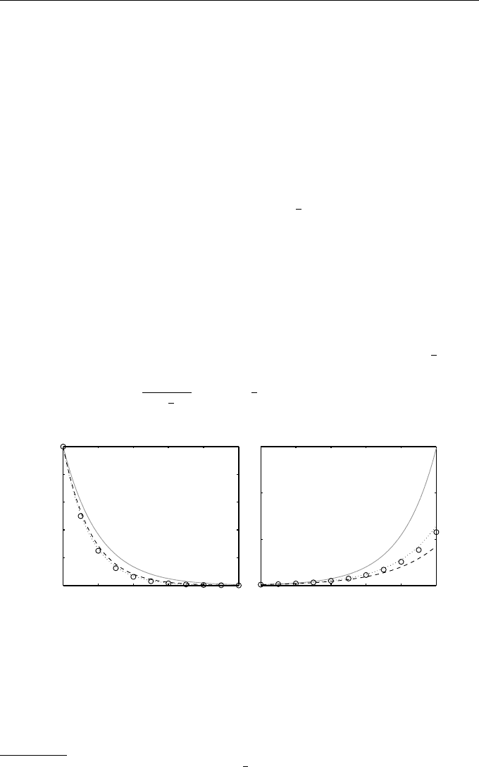
This is borne out in Figure 13.1, where we show the solution of the original

problem x(t) (solid curve), the solution of the modiﬁed equation y(t) (dashed

curve), and the numerical solution x

with h = 0.1 (circles), λ = −5 (left), and

λ = 5 (right).

We easily c alculate in this example that x(t) = e

λt

and y(t) = e

µt

. When

λ ∈ R it can be shown that µ < λ so long as 1 +

λh > 0 (which will always be

the case if h is suﬃciently small). Hence, if λ < 0, y(t) (and therefore also x

)

will decay faster than x(t) (see Figure 13.1, left). Contrariwise, when λ > 0,

y(t) (and x

) will increase more slowly than x(t) (see Figure 13.1, right)—in

both cases one could say that Euler’s m ethod introduces too much damping.

It is possible, as described in Exercise 13.3, to derive a modiﬁed equation that

approximates the numerical method to higher orders. The solutions of such a

method of order 3 are shown as dotted curves in Figure 13.1.

By retaining the ﬁrst two terms in the binomial expansion

of (1 +

λh)

−1

1 +

λh

= λ(1 −

λh) + O(h

0 0.2 0.4 0.6 0.8 1

0.2

0.4

0.6

0.8

x, y

0 0.2 0.4 0.6 0.8 1

100

150

Fig. 13.1 The circles show the numerical solutions for Example 13.1 with

h = 0.1, λ = −5 (left), and λ = 5 (right). The solid curve shows the solution

x(t) of the original ODE x

(t) = λx(t), the dashed curve y(t) the solution of

the modiﬁed Equation (13.6) and the dotted curve the solution of the modiﬁed

equation of order 3 given in Exercise 13.3

We use p = −1 in (1 + z)

= 1 + pz +

p(p − 1)z

+ . . . (which is convergent for

|z| < 1) and retain only the ﬁrst two terms. See, for example, [12, 64].

13.2 One-Step Methods 181

we are led to an alternative modiﬁed equation

(t) = µy(t), µ =

1 +

λh

, (13.8)

with which the numerical method is also consistent of second order. This illus-

trates the non-uniqueness of modiﬁed equations. It also allows us to demon-

strate the important principal that one cannot deduce stability properties of a

numerical method by analysing its modiﬁed equation(s). Here, when λ < 0, the

solutions to the original modiﬁed Equation (13.6) decay to zero for all h > 0,

since µ < 0. For the alternative modiﬁed Equation (13.8), µ < 0 only for those

step sizes h for which 1 +

hλ > 0. Thus the two possible modiﬁed equations

have quite diﬀerent behaviours when h is too large. So the concept is only

relevant for suﬃciently small h.

Example 13.2

Use modiﬁed equations to compare the behaviour of forward and backward

Euler methods for solving the logistic equation x

(t) = 2x(t)



1 − x(t)



with

initial condition x(0) = 0.1.

With f(y) = 2y(1 − y), the modiﬁed equation (13.5) for Euler’s method

becomes

(t) =



1 − hy(1 − 2y)



y(1 − y), (13.9)

while that for the backward Euler method is (see Exercise 13.5)

(t) =



1 + hy(1 − 2y)



y(1 − y), (13.10)

the initial condition being y(0) = 0.1 in both cases. The right-hand sides of both

these e quations are positive for 0 < y < 1 and h < 1, so the corresponding

IVPs have monotonically increasing solutions.

For 0.5 < y < 1 the solution y(t) of (13.9) satisﬁes y

(t) < y(1 − y), so the

solution of the modiﬁed equation (and, therefore, the solution of the forward

Euler method) increases more slowly than the exact solution x(t), while, for

0.5 < y < 1, y

(t) > y(1 − y) and the numerical solution grows more quickly.

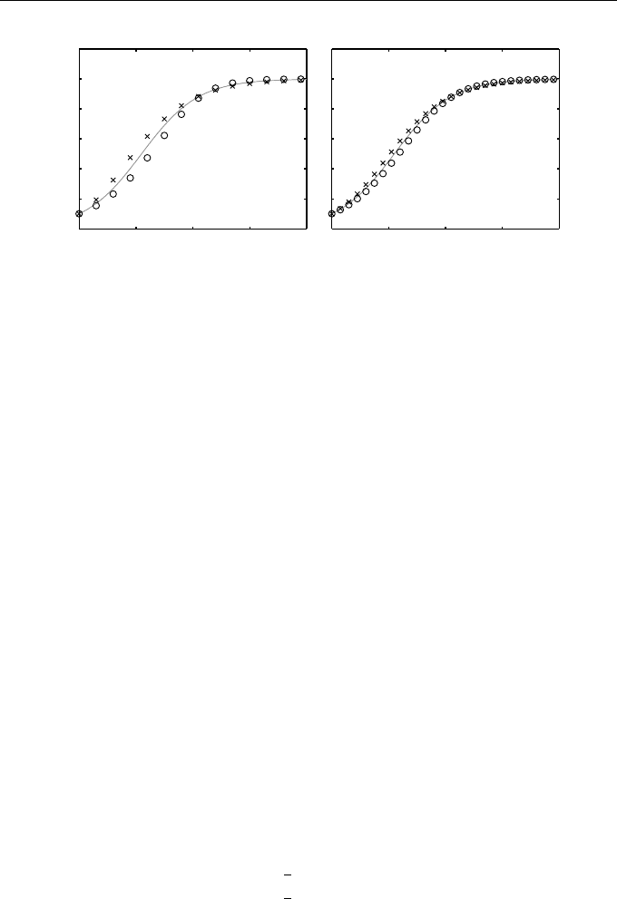
These properties are reversed for Equation (13.10) and the backward Euler

method. These deductions are conﬁrmed by the numerical results shown in

Figure 13.2 with h = 0.3 and h = 0.15.

In our next example we stay with Euler’s method, but this time it is applied

to a system of ODEs. The steps involved in the construction of a modiﬁed

system of equations are similar to those in Example 13.1, except that vector

quantities are involved.

182 13. Modiﬁed Equations

0 1 2 3 4

0.2

0.4

0.6

0.8

0 1 2 3 4

0.2

0.4

0.6

0.8

Fig. 13.2 Numerical solutions of the logistic equation with the forward Euler

method (circles) and backward Euler method (crosses) of Example 13.2 with

h = 0.3 (left) and h = 0.15 (right). Also shown is the exact solution x(t) of the

IVP (solid curve)

Example 13.3

Euler’s method applied to the IVP

(t) = −v(t), v

(t) = u(t),

u(0) = 1, v(0) = 0

(13.11)

leads to

n+1

= u

− hv

, v

n+1

= v

+ hu

, n = 0, 1, . . . ,

= 1, v

= 0,

(13.12)

and the numerical solutions with h = 1/2 are displayed on the left of Figure 7.3.

Derive a modiﬁed system of equations that will capture the behaviour of the

numerical solution.

We suppose that the modiﬁed equation is a system of two ODEs with de-

pendent variables x(t) and y(t). The LTE of the given method is, therefore,

n+1



x(t + h) − x(t) + hy(t)

y(t + h) − y(t) − hx(t)



, t = nh, (13.13)

which, by Taylor expansion, becomes

n+1

= h



(t) +

(t) + y(t)

(t) +

(t) − x(t)



+ O(h

). (13.14)

We now suppose that the modiﬁed equations take the form

(t) = −y(t) + ha(x, y),

(t) = x(t) + hb(x, y),

13.2 One-Step Methods 183

where the functions a(x, y) and b(x, y) are to be determined. Diﬀerentiating

these with respect to t gives

(t) = −y

(t) + O(h) = −x(t) + O(h),

(t) = x

(t) + O(h) = −y(t) + O(h).

Substitution into (13.14) then leads to

n+1

= h



a(x, y) −

x(t)

b(x, y) −

y(t)



+ O(h

Therefore,

n+1

= O(h

) on choosing a(x, y) =

x and b(x, y) =

y. Our

modiﬁed system of equations is, therefore,

(t) = −y(t) +

hx(t),

(t) = x(t) +

hy(t).

(13.15)

They can be written in matrix-vector form as (see also Exercise 13.6)

(t) =

Ax(t), x(t) =



x(t)

y(t)



A =



h −1



. (13.16)

When x(t) and y(t) satisfy these ODEs the LTE (13.13) is of order O(h

) and

so Euler’s method must be convergent to x(t) of order 2. That is, the solutions

of (13.12) satisfy

= x(t

) + O(h

), v

= y(t

) + O(h

In order to use these modiﬁed equations to explain the behaviour of numer-

ical solutions observed in Example 7.6 (see Figure 7.3, left), we observe that

the eigenvalues of the matrix A in (13.16) are given by

h ± i.

These have (small) positive real parts, which means that the solutions in the

phase plane will spiral outwards. This behaviour can be quantiﬁed w ithout

having to solve the modiﬁed system; it can be deduced (the details are left to

Exercise 13.8) that

(t) + y

(t) = e

. (13.17)

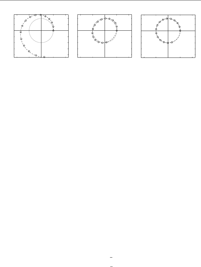
The curve described by this equation is a s piral and is shown in Figure 13.3 as

a dashed line that accurately predicts the behaviour of the numerical solution

(shown as dots) when h = 1/3 (such a large step size is used for illustrative

purp ose s).

The behaviour of Euler’s method in the previous example was clearly in-

appropriate for dealing with an oscillatory problem (characterized by solutions

184 13. Modiﬁed Equations

−2 −1 0 1 2

−2

−1.5

−1

−0.5

0.5

−2 −1 0 1 2

−2

−1.5

−1

−0.5

0.5

−2 −1 0 1 2

−2

−1.5

−1

−0.5

0.5

Fig. 13.3 Left: the numerical solutions for Example 13.3 for 0 ≤ t ≤ 5. The

dots show the solution of (13.12) with h = 1/3 in the u-v phase plane; the

solid curve is the circular trajectory of the original IVP and the dashed line

the solution of the modiﬁed Equation (13.16). In the centre and on the right

are shown the corresponding results for Examples 13.4 and 13.5

forming closed curves in the phase plane). We show in the next two exam-

ples how small modiﬁcations of the method lead to a dramatic improvement in

performance.

In the ﬁrst variation of Euler’s method, the usual “forward Euler” (FE)

method is applied to the ﬁrst ODE of the system (13.11) while the backward

version (BE) is applied to the second equation.

Example 13.4 (The Symplectic Euler Method)

Derive a modiﬁed system of equations that will describe the behaviour of so-

lutions of the method

FE : u

n+1

= u

− hv

BE : v

n+1

= v

+ hu

n+1

(13.18)

for the IVP (13.11) from the previous example.

Following the same steps as the previous example it can be shown that,

instead of (13.15), we arrive at

(t) = −y(t) +

hx(t)

(t) = x(t) −

hy(t)

)

, (13.19)

which diﬀers from (13.15) in that the sign of y(t) on the right-hand side of the

second equation has changed. It is now possible to deduce that the trajectories

in the phase plane lie on one of the family of ellipses

(t) − hx(t)y(t) + y

(t) = constant (13.20)

(see Exercise 13.9). In this particular case the initial conditions x(0) = 1,

y(0) = 0 ﬁx the constant term to be 1. This ellipse is shown in Figure 13.3

13.2 One-Step Methods 185

(centre) as a dashed curve. The numerically computed points (u

, v

) lie, to

within graphical accuracy, exactly on this ellipse. As h → 0 the ellipse collapses

to the circle x

(t) + y

(t) = 1 (shown as a solid curve), which is the trajectory

followed by the exact solution of the original equations (see Example 13.1).

Because the numerical solutions follow closed orbits the method is well suited

to integration of the system over long time intervals. This result would not

be signiﬁcant if it held only for this linear system of diﬀerential equations,

since it can be solved exactly and there is no practical need for a numerical

method. However, the method generalizes quite simply to nonlinear situations,

as described in Exercise 13.11. This method is also discussed in a more general

context in Section 15.3.

The symplectic Euler method (13.18) oﬀers a signiﬁcant improvement over

the standard Euler method but it is still only a ﬁrst-order accurate method.

The second variation of Euler’s method leads to a s econd-order method. In

its basic form it begins by applying the symplectic Euler method with a step

size h/2 and then repeats the process with the order of the ODEs reversed.

This removes the bias present in the symplectic Euler method (FE is always

applied before BE). The use of half step sizes h/2 necessitates the introduction

of quantities such as u

n−

and u

(known as “half-integer” values) which

approximate solutions, respectively, at times t = (n−

)h and (n+

)h, midway

between the points t = t

n−1

, t = t

and t = t

n+1

on the temporal grid.

Example 13.5 (The St¨ormer–Verlet Method)

Derive a modiﬁed system of equations that will describe the behaviour of so-

lutions of the method

FE : u

= u

−

BE : v

= v

FE : v

n+1

= v

)

BE : u

n+1

= u

−

n+1

= v

+ hu

(13.21)

for the IVP (13.11) from the previous example.

As indicated, the middle two stages may be combined into one. Further

computational savings can be achieved by also combining the last stage of one

step with the ﬁrst step of the next stage. Thus, for computational purp os es,

the algorithm involves:

1. u

= u

−

and v

= v

+ hu

2. u

= u

n−

+ hv

and v

n+1

= v

+ hu

for n = 1, 2, . . . .